Randomly Split a Graph into Mini Graphs

Question

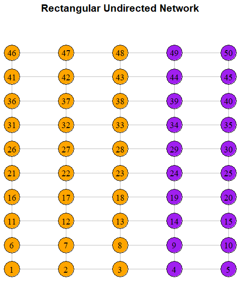
I have this graph network in R:

library(igraph)
n_rows <- 10
n_cols <- 5
g <- make_lattice(dimvector = c(n_cols, n_rows))

layout <- layout_on_grid(g, width = n_cols)

n_nodes <- vcount(g)
node_colors <- rep("white", n_nodes)

for (row in 0:(n_rows-1)) {
    start_index <- row * n_cols + 1
    node_colors[start_index:(start_index+2)] <- "orange"  
    node_colors[(start_index+3):(start_index+4)] <- "purple"    
}

node_labels <- 1:n_nodes

plot(g, 
     layout = layout, 
     vertex.color = node_colors,
     vertex.label = node_labels,
     vertex.label.color = "black",
     vertex.size = 15,
     edge.color = "gray",
     main = "Rectangular Undirected Network")

I am trying to write a function which randomly breaks this network into 5 connected subgraphs (i.e. mini graphs) such that each node appears exactly once.

I think in theory, this should not be too difficult to do. I would need to randomly identify a node, randomly decide how many neighbors to include, select those neighbors and remove them from the graph .... and restart this process on the remaining graph. Of course, some additional details would need to be specified, e.g. if the random number specified exceed the number of remaining nodes then use a max function, BFS would need to be used to select the nodes, etc.

Here was my first attempt at writing the code:

get_connected_subgraph <- function(graph, available_nodes, min_nodes = 5, max_nodes = 15) {
    if (length(available_nodes) == 0) return(NULL)
    
    start_node <- sample(available_nodes, 1)
    
    bfs_result <- bfs(graph, root = start_node, unreachable = FALSE, order = TRUE, rank = TRUE, father = TRUE)
    
    bfs_order <- intersect(bfs_result$order, available_nodes)
    
    n_subgraph_nodes <- min(sample(min_nodes:max_nodes, 1), length(bfs_order))
    
    subgraph_nodes <- bfs_order[1:n_subgraph_nodes]
    
    return(subgraph_nodes)
}

create_5_subgraphs <- function(graph) {
    available_nodes <- V(graph)
    subgraphs <- list()
    
    for (i in 1:5) {
        subgraph_nodes <- get_connected_subgraph(graph, available_nodes)
        if (is.null(subgraph_nodes)) break
        
        subgraphs[[i]] <- subgraph_nodes
        available_nodes <- setdiff(available_nodes, subgraph_nodes)
    }
    
    return(subgraphs)
}

set.seed(42) 
subgraphs <- create_5_subgraphs(g)

subgraph_colors <- c("red", "blue", "green", "yellow", "purple")

node_subgraph_colors <- rep("lightgray", vcount(g))
for (i in 1:length(subgraphs)) {
    node_subgraph_colors[subgraphs[[i]]] <- subgraph_colors[i]
}

edge_subgraph_colors <- rep("lightgray", ecount(g))
for (i in 1:length(subgraphs)) {
    subgraph_edges <- E(g)[.inc(subgraphs[[i]])]
    edge_subgraph_colors[subgraph_edges] <- subgraph_colors[i]
}

plot(g, 
     layout = layout,
     vertex.color = node_subgraph_colors,
     vertex.label = node_labels,
     vertex.label.color = "black",
     vertex.size = 15,
     edge.color = edge_subgraph_colors,
     edge.width = 2,
     main = "Network with 5 Separate Connected Subgraphs")

The above result looks almost correct, but the yellow nodes (e.g. 29) appears to be violating the connectivity.

Any pointers on how to fix this?

---

I wrote some optional code to compare the before/after:

node_info <- data.frame(
    Node_Index = 1:vcount(g),
    Original_Color = node_colors,
    New_Color = node_subgraph_colors
)

get_subgraph_number <- function(node) {
    subgraph_num <- which(sapply(subgraphs, function(x) node %in% x))
    if (length(subgraph_num) == 0) return(NA)
    return(subgraph_num)
}

node_info$Subgraph_Number <- sapply(node_info$Node_Index, get_subgraph_number)

head(node_info)

---

To complement jblood94's amazing answer, here is a quick plotting function that works with jblood94's answer:

library(igraph)
library(data.table)

f <- function(g, n) {
    m <- length(g)
    dt <- setDT(as_data_frame(g))
    dt <- rbindlist(list(dt, dt[,.(from = to, to = from)]))
    dt[,group := 0L]
    used <- logical(m)
    s <- sample(m, n)
    used[s] <- TRUE
    m <- m - n
    dt[from %in% s, group := .GRP, from]
    
    while (m) {
        dt2 <- unique(
            dt[group != 0L & !used[to], .(grow = to, onto = group)][sample(.N)],
            by = "grow"
        )
        dt[dt2, on = .(from = grow), group := onto]
        used[dt2[[1]]] <- TRUE
        m <- m - nrow(dt2)
    }
    
    unique(dt[,to := NULL])[,.(vertices = .(from)), group]
}


plot_multiple_subgraphs <- function(n_plots = 25, n_rows = 10, n_cols = 5, n_subgraphs = 5) {
    g <- make_lattice(dimvector = c(n_cols, n_rows))
    layout <- layout_on_grid(g, width = n_cols)
    n_nodes <- vcount(g)
    
    color_palette <- c("red", "blue", "green", "yellow", "purple")
    
    par(mfrow = c(5, 5), mar = c(0.5, 0.5, 2, 0.5))
    
    for (i in 1:n_plots) {
        subgraphs <- f(g, n_subgraphs)
        
        node_colors <- rep("white", n_nodes)
        
        for (j in 1:nrow(subgraphs)) {
            nodes <- unlist(subgraphs$vertices[j])
            node_colors[nodes] <- color_palette[j]
        }
        
        plot(g, 
             layout = layout, 
             vertex.color = node_colors,
             vertex.label = NA,  
             vertex.size = 15,   
             edge.color = "gray",
             edge.width = 0.5,  
             main = paste("Partition", i),  
             cex.main = 0.8)     
    }
}

plot_multiple_subgraphs()

Kovar

If you don't need the subgraph size constraints you can just delete edges until count_components(g_sub) == 5. I think your problem is that you're doing BFS on the original graph and taking the intersection with remaining nodes. You might first create a new graph that only has available vertices and BFS that. – Veracity

@n1000: thank you so much! by size constraint, you mean ... minimum size of each subgraph? – Kovar

Yes. I took min_nodes=5 to be a restriction on the allowed subgraph partitions. – Veracity

Does this mimic the minimal code to reproduce your issue? – Cannelloni

Answer 1

Here's a function that randomly selects n vertices from the graph g as the initial subgraph member for each of n groups, then iteratively "grows" each group until all the vertices are in a subgraph.

library(data.table)

f <- function(g, n) {
  m <- length(g)
  dt <- setDT(as_data_frame(g))
  dt <- rbindlist(list(dt, dt[,.(from = to, to = from)]))
  dt[,group := 0L]
  used <- logical(m)
  s <- sample(m, n)
  used[s] <- TRUE
  m <- m - n
  dt[from %in% s, group := .GRP, from]
  
  while (m) {
    dt2 <- unique(
      dt[group != 0L & !used[to], .(grow = to, onto = group)][sample(.N)],
      by = "grow"
    )
    dt[dt2, on = .(from = grow), group := onto]
    used[dt2[[1]]] <- TRUE
    m <- m - nrow(dt2)
  }
  
  unique(dt[,to := NULL])[,.(vertices = .(from), .N), group]
}

Demonstrating on the OP's graph:

set.seed(907044864)
f(g, 5L)
#>    group              vertices     N
#>    <int>                <list> <int>
#> 1:     1       1,2,3,6,7,8,...     9
#> 2:     2  4, 5, 9,10,13,14,...    13
#> 3:     3 21,22,26,27,31,36,...     9
#> 4:     4 23,28,29,32,33,38,...    10
#> 5:     5 30,34,35,39,40,44,...     9

Note: during the iterations, if multiple groups try to "grow into" the same vertex, the winning group is selected randomly. This is done with [sample(.N)] after all the candidate growths are found with dt[group != 0L & !used[to], .(grow = to, onto = group)].

---

Performance check

Testing performance on partitioning a 100-by-100 grid into 10 groups:

system.time(dt <- f(make_lattice(c(100, 100)), 10))
#>    user  system elapsed 
#>    0.16    0.02    0.17
dt
#>     group                          vertices     N
#>     <int>                            <list> <int>
#>  1:     4                   1,2,3,4,5,6,...  2329
#>  2:     2             43,44,45,46,47,48,...  1093
#>  3:     1             87,88,89,90,91,92,...    99
#>  4:     3       695,696,697,795,796,797,...   380
#>  5:     5 1551,1552,1553,1554,1650,1651,...  1363
#>  6:     6 3171,3172,3173,3174,3175,3176,...  1048
#>  7:     7 5921,5922,5923,5924,5925,5926,...  2377
#>  8:     8 6169,6171,6269,6270,6271,6272,...   339
#>  9:     9 6475,6575,6576,6675,6676,6677,...   264
#> 10:    10 7980,7981,7982,7983,7984,7985,...   708

Magree

thank you so much! I posted a visualization code as an extra – Kovar

Nice! I wanted to see what the partitions were looking like, but didn't feel like coding up the visualization. – Magree

@jbllod94: Do you have any ideas about this question here? https://mcmap.net/q/2031185/-fading-colors-in-a-graph – Kovar

Answer 2

With igraph::voronoi_cells(g, ...)$membership:

library(igraph, warn.conflicts = FALSE)

n_rows <- 10
n_cols <- 5

g <- make_lattice(dimvector = c(n_cols, n_rows))

# Voronoi partitioning
set.seed(42)
V(g)$sub <- voronoi_cells(g, sample(V(g), 5), tiebreaker = "first")$membership

# summary
V(g)$names <- V(g)
as_data_frame(g, what = "vertices") |> 
  dplyr::summarise(names = list(names), size = lengths(names), .by = sub)
#>   sub                                                  names size
#> 1   2                              1, 2, 3, 6, 7, 11, 12, 16    8
#> 2   4                             4, 5, 8, 9, 10, 13, 14, 15    8
#> 3   1 17, 21, 22, 26, 27, 28, 31, 32, 33, 36, 37, 38, 41, 42   14
#> 4   3                     18, 19, 20, 23, 24, 25, 29, 30, 35    9
#> 5   0             34, 39, 40, 43, 44, 45, 46, 47, 48, 49, 50   11

withr::with_par(
  list(mar = c(0, 0, 0, 0)),
  plot(g, 
       layout = layout_on_grid(g, width = n_cols), 
       # membership IDs are 0-based, hence +1 to subset colors
       vertex.color = c("red", "blue", "green", "yellow", "purple")[V(g)$sub + 1],
       vertex.label.color = "black",
       vertex.size = 15,
       edge.color = "gray")
)

^{Created on 2024-09-13 with reprex v2.1.1}

Issus

@margsul: thank you! I thought voroni diagrams are deterministic ? – Kovar

With a constant generator vector (order plays a role too) and non-random tiebreaker they are (random might not play nice with small graphs) . Do you need it to be random when called with the same sequence of nodes? – Issus

Answer 3

I would say that your bfs is a good approach to start from, and you can use bfs like below

nrsubg <- 5
gg <- g <- g %>%
  set_vertex_attr("name", value = seq.int(vcount(.)))
szsubg <- diff(sort(c(0, vcount(g), sample(vcount(g) - 1, nrsubg - 1))))
vlst <- setNames(vector("list", nrsubg), seq.int(nrsubg))
for (i in seq_along(szsubg)) {
  vlst[[i]] <- names(head(bfs(gg, sample(V(gg)[which.min(degree(gg))], 1))$order, szsubg[i]))
  gg <- induced_subgraph(gg, V(gg)[!names(V(gg)) %in% vlst[[i]]])
}
g %>%
  set_vertex_attr("color", value = with(stack(vlst), ind[match(names(V(.)), values)])) 

where the size of each connected "mini graph" is random.

visualization

g %>% 
  plot(
    layout = layout,
    vertex.label = V(.)$name,
    vertex.label.color = "black",
    vertex.size = 15,
    edge.color = "gray",
    main = "Rectangular Undirected Network"
  )

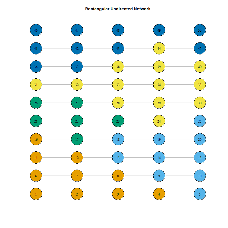
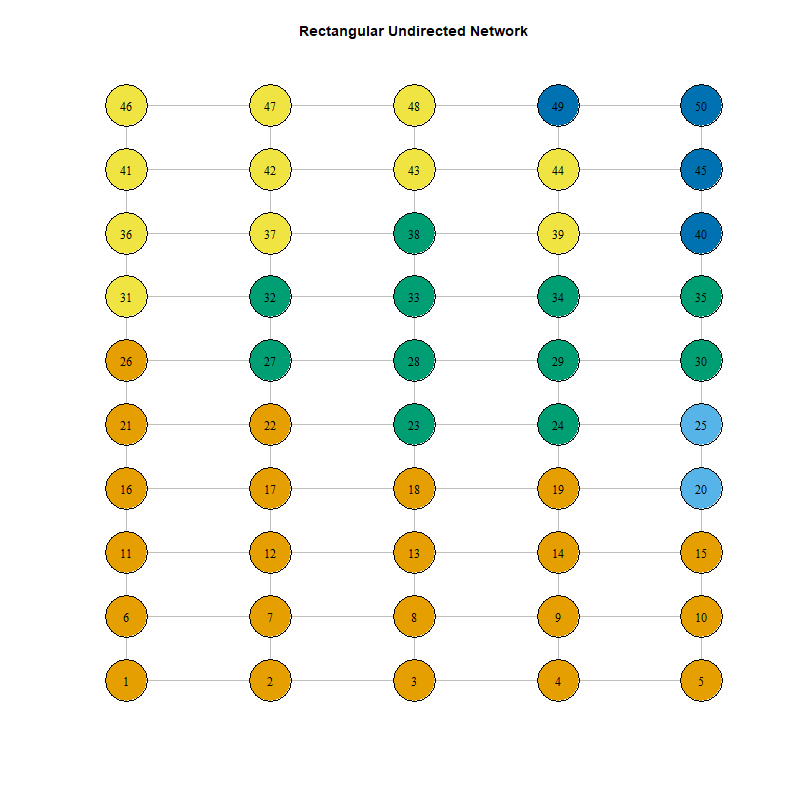
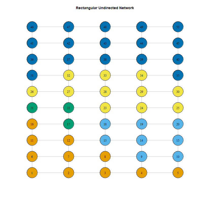
shows something like below for example

Granadilla

Thank you so much for this cool answer! Do you have any idea about this one here? https://mcmap.net/q/2031185/-fading-colors-in-a-graph – Kovar