Minimum Cost Flow - network optimization in R

Question

I am trying to implement a "Minimum Cost Network Flow" transportation problem solution in R.

I understand that this could be implemented from scratch using something like lpSolve. However, I see that there is a convenient igraph implementation for "Maximum Flow". Such a pre-existing solution would be a lot more convenient, but I can't find an equivalent function for Minimum Cost.

Is there an igraph function that calculates Minimum Cost Network Flow solutions, or is there a way to apply the igraph::max_flow function to a Minimum Cost problem?

igraph network example:

library(tidyverse)
library(igraph)

edgelist <- data.frame(
  from = c(1, 1, 2, 2, 2, 3, 3, 3, 4, 4, 5, 5, 6, 6, 7, 8),
  to = c(2, 3, 4, 5, 6, 4, 5, 6, 7, 8, 7, 8, 7, 8, 9, 9),
  capacity = c(20, 30, 99, 99, 99, 99, 99, 99, 99, 99, 99, 99, 99, 99, 99, 99),
  cost = c(0, 0, 1, 2, 3, 4, 3, 2, 3, 2, 3, 4, 5, 6, 0, 0))

g <- graph_from_edgelist(as.matrix(edgelist[,c('from','to')]))

E(g)$capacity <- edgelist$capacity
E(g)$cost <- edgelist$cost

plot(g, edge.label = E(g)$capacity)
plot(g, edge.label = E(g)$cost)

This is a network with directional edges, a "source node" (1), and a "sink node" (9). Each edge has a "capacity" (here often put as 99 for unlimited) and a "cost" (the cost of one unit flowing through this edge). I want to find the integer vector of flows (x, length = 9) that minimises the cost while transmitting a pre-defined flow through the network (let's say 50 units, from node 1 into node 9).

Disclaimer: this post asked a similar question, but did not result in a satisfying answer and is rather dated (2012).

Gimcrack

Which are the desired result? Im looking for a answer but need to see if match with your answer – Cassandracassandre

Thanks gonzalez.ivan90! The desired output is something similar to the output of the max_flow function, but for a minimum cost flow rather than a maximum flow. This would be a vector of weights (x) that quantifies the optimal (minimum cost) flow across all edges of the network. It's tricky to provide example code because my question is basically: "Can I get around the massive pain of writing all of this into an lpSolve value and constraint matrix?". Hope this clarifies the problem? – Gimcrack

I pefer the result. My scritp have this partition2 output: + 3/6 vertices, named: 3 4 2 This is the minimum cost path? – Cassandracassandre

Your code does not work under R 3.4.1, Win64, igraph_1.1.2. Could you please correct it? Thanks! – Astronautics

@StephanKolassa updated both the example and my answer. Works for me, can you let me know if it does for you? Cheers! – Gimcrack

My R can't find data_frame()... can you perhaps start with a completely new and empty instance of R (that does not read any custom startup scripts that may already library or require certain packages) and tweak your code until it runs successfully? Thanks! – Astronautics

data_frame should be in the tidyverse package, which I included in my example. This particular bit of the code actually runs without the tidyverse version, using data.frame instead. You will, however, need other tidyverse functions to run my code in the answer below. – Gimcrack

Answer 1

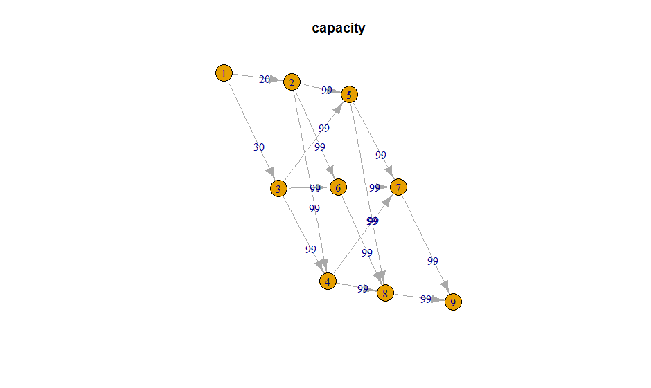
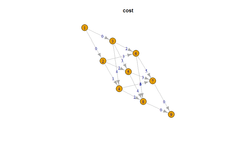
In case of interest, here is how I ended up solving this problem. I used an edge dataframe with to nodes, from nodes, cost property and capacity property for each edge to create a constraint matrix. Subsequently, I fed this into a linear optimisation using the lpSolve package. Step-by-step below.

---

Start with the edgelist dataframe from my example above

library(magrittr)

# Add edge ID
edgelist$ID <- seq(1, nrow(edgelist))

glimpse(edgelist)

Looks like this:

Observations: 16
Variables: 4
$ from     <dbl> 1, 1, 2, 2, 2, 3, 3, 3, 4, 4, 5, 5, 6, 6, 7, 8
$ to       <dbl> 2, 3, 4, 5, 6, 4, 5, 6, 7, 8, 7, 8, 7, 8, 9, 9
$ capacity <dbl> 20, 30, 99, 99, 99, 99, 99, 99, 99, 99, 99, 99, 99, 99, 99, 99
$ cost     <dbl> 0, 0, 1, 2, 3, 4, 3, 2, 3, 2, 3, 4, 5, 6, 0, 0
$ ID       <int> 1, 2, 3, 4, 5, 6, 7, 8, 9, 10, 11, 12, 13, 14, 15, 16

---

Create constraints matrix

createConstraintsMatrix <- function(edges, total_flow) {

  # Edge IDs to be used as names
  names_edges <- edges$ID
  # Number of edges
  numberof_edges <- length(names_edges)

  # Node IDs to be used as names
  names_nodes <- c(edges$from, edges$to) %>% unique
  # Number of nodes
  numberof_nodes <- length(names_nodes)

  # Build constraints matrix
  constraints <- list(
    lhs = NA,
    dir = NA,
    rhs = NA)

  #' Build capacity constraints ------------------------------------------------
  #' Flow through each edge should not be larger than capacity.
  #' We create one constraint for each edge. All coefficients zero
  #' except the ones of the edge in question as one, with a constraint
  #' that the result is smaller than or equal to capacity of that edge.

  # Flow through individual edges
  constraints$lhs <- edges$ID %>%
    length %>%
    diag %>%
    set_colnames(edges$ID) %>%
    set_rownames(edges$ID)
  # should be smaller than or equal to
  constraints$dir <- rep('<=', times = nrow(edges))
  # than capacity
  constraints$rhs <- edges$capacity


  #' Build node flow constraints -----------------------------------------------
  #' For each node, find all edges that go to that node
  #' and all edges that go from that node. The sum of all inputs
  #' and all outputs should be zero. So we set inbound edge coefficients as 1
  #' and outbound coefficients as -1. In any viable solution the result should
  #' be equal to zero.

  nodeflow <- matrix(0,
                     nrow = numberof_nodes,
                     ncol = numberof_edges,
                     dimnames = list(names_nodes, names_edges))

  for (i in names_nodes) {

    # input arcs
    edges_in <- edges %>%
      filter(to == i) %>%
      select(ID) %>%
      unlist
    # output arcs
    edges_out <- edges %>%
      filter(from == i) %>%
      select(ID) %>%
      unlist

    # set input coefficients to 1
    nodeflow[
      rownames(nodeflow) == i,
      colnames(nodeflow) %in% edges_in] <- 1

    # set output coefficients to -1
    nodeflow[
      rownames(nodeflow) == i,
      colnames(nodeflow) %in% edges_out] <- -1
  }

  # But exclude source and target edges
  # as the zero-sum flow constraint does not apply to these!
  # Source node is assumed to be the one with the minimum ID number
  # Sink node is assumed to be the one with the maximum ID number
  sourcenode_id <- min(edges$from)
  targetnode_id <- max(edges$to)
  # Keep node flow values for separate step below
  nodeflow_source <- nodeflow[rownames(nodeflow) == sourcenode_id,]
  nodeflow_target <- nodeflow[rownames(nodeflow) == targetnode_id,]
  # Exclude them from node flow here
  nodeflow <- nodeflow[!rownames(nodeflow) %in% c(sourcenode_id, targetnode_id),]

  # Add nodeflow to the constraints list
  constraints$lhs <- rbind(constraints$lhs, nodeflow)
  constraints$dir <- c(constraints$dir, rep('==', times = nrow(nodeflow)))
  constraints$rhs <- c(constraints$rhs, rep(0, times = nrow(nodeflow)))


  #' Build initialisation constraints ------------------------------------------
  #' For the source and the target node, we want all outbound nodes and
  #' all inbound nodes to be equal to the sum of flow through the network
  #' respectively

  # Add initialisation to the constraints list
  constraints$lhs <- rbind(constraints$lhs,
                           source = nodeflow_source,
                           target = nodeflow_target)
  constraints$dir <- c(constraints$dir, rep('==', times = 2))
  # Flow should be negative for source, and positive for target
  constraints$rhs <- c(constraints$rhs, total_flow * -1, total_flow)

  return(constraints)
}

constraintsMatrix <- createConstraintsMatrix(edges, 30)

Should result in something like this

$lhs
1  2  3  4  5  6  7  8  9 10 11 12 13 14 15 16
1       1  0  0  0  0  0  0  0  0  0  0  0  0  0  0  0
2       0  1  0  0  0  0  0  0  0  0  0  0  0  0  0  0
3       0  0  1  0  0  0  0  0  0  0  0  0  0  0  0  0
4       0  0  0  1  0  0  0  0  0  0  0  0  0  0  0  0
5       0  0  0  0  1  0  0  0  0  0  0  0  0  0  0  0
6       0  0  0  0  0  1  0  0  0  0  0  0  0  0  0  0
7       0  0  0  0  0  0  1  0  0  0  0  0  0  0  0  0
8       0  0  0  0  0  0  0  1  0  0  0  0  0  0  0  0
9       0  0  0  0  0  0  0  0  1  0  0  0  0  0  0  0
10      0  0  0  0  0  0  0  0  0  1  0  0  0  0  0  0
11      0  0  0  0  0  0  0  0  0  0  1  0  0  0  0  0
12      0  0  0  0  0  0  0  0  0  0  0  1  0  0  0  0
13      0  0  0  0  0  0  0  0  0  0  0  0  1  0  0  0
14      0  0  0  0  0  0  0  0  0  0  0  0  0  1  0  0
15      0  0  0  0  0  0  0  0  0  0  0  0  0  0  1  0
16      0  0  0  0  0  0  0  0  0  0  0  0  0  0  0  1
2       1  0 -1 -1 -1  0  0  0  0  0  0  0  0  0  0  0
3       0  1  0  0  0 -1 -1 -1  0  0  0  0  0  0  0  0
4       0  0  1  0  0  1  0  0 -1 -1  0  0  0  0  0  0
5       0  0  0  1  0  0  1  0  0  0 -1 -1  0  0  0  0
6       0  0  0  0  1  0  0  1  0  0  0  0 -1 -1  0  0
7       0  0  0  0  0  0  0  0  1  0  1  0  1  0 -1  0
8       0  0  0  0  0  0  0  0  0  1  0  1  0  1  0 -1
source -1 -1  0  0  0  0  0  0  0  0  0  0  0  0  0  0
target  0  0  0  0  0  0  0  0  0  0  0  0  0  0  1  1

$dir
[1] "<=" "<=" "<=" "<=" "<=" "<=" "<=" "<=" "<=" "<=" "<=" "<=" "<=" "<="
[15] "<=" "<=" "==" "==" "==" "==" "==" "==" "==" "==" "=="

$rhs
[1]  20  30  99  99  99  99  99  99  99  99  99  99  99  99  99  99   0
[18]   0   0   0   0   0   0 -30  30

---

Feed constraints to lpSolve for the ideal solution

library(lpSolve)

# Run lpSolve to find best solution
solution <- lp(
  direction = 'min',
  objective.in = edgelist$cost,
  const.mat = constraintsMatrix$lhs,
  const.dir = constraintsMatrix$dir,
  const.rhs = constraintsMatrix$rhs)

# Print vector of flow by edge
solution$solution

# Include solution in edge dataframe
edgelist$flow <- solution$solution

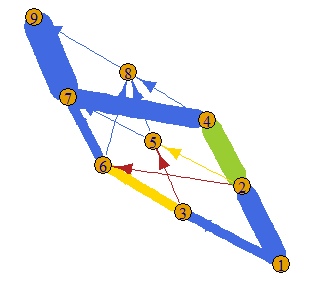
Now we can convert our edges to a graph object and plot the solution

library(igraph)

g <- edgelist %>%
  # igraph needs "from" and "to" fields in the first two colums
  select(from, to, ID, capacity, cost, flow) %>%
  # Make into graph object
  graph_from_data_frame()

# Get some colours in to visualise cost
E(g)$color[E(g)$cost == 0] <- 'royalblue'
E(g)$color[E(g)$cost == 1] <- 'yellowgreen'
E(g)$color[E(g)$cost == 2] <- 'gold'
E(g)$color[E(g)$cost >= 3] <- 'firebrick'

# Flow as edge size,
# cost as colour
plot(g, edge.width = E(g)$flow)

Hope it's interesting / useful :)

Gimcrack

This looks really interesting. I'm just a bit puzzled by the total_flow variable. Why do you need it and how do you choose one? – Pleadings

Hi @Enzo, thank you for your interest! In "minimum cost flow" the setup is that you have a total flow that you want to get through the network as cheaply as possible. For example, think factories, warehouses, stores. You know the demand for your product (total flow) and you are trying to meet demand with an optimal transportation solution (minimum cost). I've written a blog post about this that goes into some more detail in case you're interested: janlauge.github.io/2017/minimum-cost-flow-problem – Gimcrack

Answer 2

I was looking for a function but didn't success. The original function calls another: res <- .Call("R_igraph_maxflow", graph, source - 1, target - 1, capacity, PACKAGE = "igraph")

And I don't know how to deal with it.

For the moment I inverted the cost path values in order to use the same function in oposite direction:

E2 <- E # create another table
E2[, 3] <- max(E2[, 3]) + 1 - E2[, 3] # invert values

E2
     from to capacity
[1,]    1  3        8
[2,]    3  4       10
[3,]    4  2        9
[4,]    1  5       10
[5,]    5  6        9
[6,]    6  2        1

g2 <- graph_from_data_frame(as.data.frame(E2)) # create 2nd graph

# Get maximum flow
m1 <- max_flow(g1, source=V(g1)["1"], target=V(g1)["2"])
m2 <- max_flow(g2, source=V(g2)["1"], target=V(g2)["2"])

m1$partition2 # Route on maximal cost
+ 4/6 vertices, named:
[1] 4 5 6 2

m2$partition2 # Route on minimal cost
+ 3/6 vertices, named:
[1] 3 4 2

I draw in paper the graph and my code agree with manual solution This method should be tested with real know values, as I mentioned in the comment

Cassandracassandre

I've tried your solution, but unfortunately I can't see it taking into account the "cost" of using a particular edge. Is there something I am missing? I've updated my question with a more reproducible example. – Gimcrack

Is the route 1 -> 2 -> 4 -> 8 -> 9 the "Minimum Cost Network Flow"? – Cassandracassandre

In my example, we have a total flow of 50 units. 1 -> 2 only has capacity for 20 units, so the remaining 30 units needs to go through 0 -> 3. The "Minimum Cost Network Flow" of the example would be: [20 units via] 1 -> 2 -> 4 -> 8 -> 9, [30 units via] 1 -> 3 -> 6 -> 8 -> 9 – Gimcrack

FYI, see below the approach that I ended up implementing. Perhaps it's interesting / useful? – Gimcrack