Maximum Active Drawdown in python

Question

I recently asked a question about calculating maximum drawdown where Alexander gave a very succinct and efficient way of calculating it with DataFrame methods in pandas.

I wanted to follow up by asking how others are calculating maximum active drawdown?

This calculates Max Drawdown. NOT! Max Active Drawdown

This is what I implemented for max drawdown based on Alexander's answer to question linked above:

def max_drawdown_absolute(returns):
    r = returns.add(1).cumprod()
    dd = r.div(r.cummax()).sub(1)
    mdd = dd.min()
    end = dd.argmin()
    start = r.loc[:end].argmax()
    return mdd, start, end

It takes a return series and gives back the max_drawdown along with the indices for which the drawdown occured.

We start by generating a series of cumulative returns to act as a return index.

r = returns.add(1).cumprod()

At each point in time, the current drawdown is calcualted by comparing the current level of the return index with the maximum return index for all periods prior.

dd = r.div(r.cummax()).sub(1)

The max drawdown is then just the minimum of all the calculated drawdowns.

My question:

I wanted to follow up by asking how others are calculating maximum active drawdown?

Assumes that the solution will extend on the solution above.

Hypogastrium

Answer 1

Starting with a series of portfolio returns and benchmark returns, we build cumulative returns for both. the variables below are assumed to already be in cumulative return space.

The active return from period j to period i is:

Solution

This is how we can extend the absolute solution:

def max_draw_down_relative(p, b):
    p = p.add(1).cumprod()
    b = b.add(1).cumprod()
    pmb = p - b
    cam = pmb.expanding(min_periods=1).apply(lambda x: x.argmax())
    p0 = pd.Series(p.iloc[cam.values.astype(int)].values, index=p.index)
    b0 = pd.Series(b.iloc[cam.values.astype(int)].values, index=b.index)
    dd = (p * b0 - b * p0) / (p0 * b0)
    mdd = dd.min()
    end = dd.argmin()
    start = cam.ix[end]
    return mdd, start, end

Explanation

Similar to the absolute case, at each point in time, we want to know what the maximum cumulative active return has been up to that point. We get this series of cumulative active returns with p - b. The difference is that we want to keep track of what the p and b were at this time and not the difference itself.

So, we generate a series of 'whens' captured in cam (cumulative argmax) and subsequent series of portfolio and benchmark values at those 'whens'.

    p0 = pd.Series(p.ix[cam.values.astype(int)].values, index=p.index)
    b0 = pd.Series(b.ix[cam.values.astype(int)].values, index=b.index)

The drawdown caclulation can now be made analogously using the formula above:

    dd = (p * b0 - b * p0) / (p0 * b0)

Demonstration

import numpy as np
import pandas as pd
import matplotlib.pyplot as plt

np.random.seed(314)
p = pd.Series(np.random.randn(200) / 100 + 0.001)
b = pd.Series(np.random.randn(200) / 100 + 0.001)

keys = ['Portfolio', 'Benchmark']
cum = pd.concat([p, b], axis=1, keys=keys).add(1).cumprod()
cum['Active'] = cum.Portfolio - cum.Benchmark


mdd, sd, ed = max_draw_down_relative(p, b)

f, a = plt.subplots(2, 1, figsize=[8, 10])

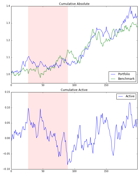
cum[['Portfolio', 'Benchmark']].plot(title='Cumulative Absolute', ax=a[0])
a[0].axvspan(sd, ed, alpha=0.1, color='r')

cum[['Active']].plot(title='Cumulative Active', ax=a[1])
a[1].axvspan(sd, ed, alpha=0.1, color='r')

Hypogastrium

To be accurate under all circumstance, the function needs to automatically add a zero as the first return to the portfolio and benchmark. p = pd.Series([ -.1,-.1,-.1], name='p') b = pd.Series([-.05,-.05,-.05], name='b') p = p.add(1).cumprod() b = b.add(1).cumprod() results = pd.concat([p,b], axis=1) results['cum diff'] = results['p'] - results['b'] results The result should be -0.128375. Your function returns -0.0925. – Hydrophyte

Answer 2

You may have noticed that your individual components do not equal the whole, either in an additive or geometric manner:

>>> cum.tail(1)
     Portfolio  Benchmark    Active
199   1.342179   1.280958  1.025144

This is always a troubling situation, as it indicates that some sort of leakage may be occurring in your model.

Mixing single period and multi-period attribution is always always a challenge. Part of the issue lies in the goal of the analysis, i.e. what are you trying to explain.

If you are looking at cumulative returns as is the case above, then one way you perform your analysis is as follows:

1. Ensure the portfolio returns and the benchmark returns are both excess returns, i.e. subtract the appropriate cash return for the respective period (e.g. daily, monthly, etc.).

2. Assume you have a rich uncle who lends you $100m to start your fund. Now you can think of your portfolio as three transactions, one cash and two derivative transactions: a) Invest your $100m in a cash account, conveniently earning the offer rate. b) Enter into an equity swap for $100m notional c) Enter into a swap transaction with a zero beta hedge fund, again for $100m notional.

We will conveniently assume that both swap transactions are collateralized by the cash account, and that there are no transaction costs (if only...!).

On day one, the stock index is up just over 1% (an excess return of exactly 1.00% after deducting the cash expense for the day). The uncorrelated hedge fund, however, delivered an excess return of -5%. Our fund is now at $96m.

Day two, how do we rebalance? Your calculations imply that we never do. Each is a separate portfolio that drifts on forever... For the purpose of attribution, however, I believe it makes total sense to rebalance daily, i.e. 100% to each of the two strategies.

As these are just notional exposures with ample cash collateral, we can just adjust the amounts. So instead of having $101m exposure to the equity index on day two and $95m of exposure to the hedge fund, we will instead rebalance (at zero cost) so that we have $96m of exposure to each.

How does this work in Pandas, you might ask? You've already calculated cum['Portfolio'], which is the cumulative excess growth factor for the portfolio (i.e. after deducting cash returns). If we apply the current day's excess benchmark and active returns to the prior day's portfolio growth factor, we calculate the daily rebalanced returns.

import numpy as np
import pandas as pd

np.random.seed(314)
df_returns = pd.DataFrame({
    'Portfolio': np.random.randn(200) / 100 + 0.001,
    'Benchmark': np.random.randn(200) / 100 + 0.001})
df_returns['Active'] = df.Portfolio - df.Benchmark

# Copy return dataframe shape and fill with NaNs.
df_cum = pd.DataFrame()  

# Calculate cumulative portfolio growth
df_cum['Portfolio'] = (1 + df_returns.Portfolio).cumprod()

# Calculate shifted portfolio growth factors.
portfolio_return_factors = pd.Series([1] + df_cum['Portfolio'].shift()[1:].tolist(), name='Portfolio_return_factor')

# Use portfolio return factors to calculate daily rebalanced returns.
df_cum['Benchmark'] = (df_returns.Benchmark * portfolio_return_factors).cumsum()
df_cum['Active'] = (df_returns.Active * portfolio_return_factors).cumsum()

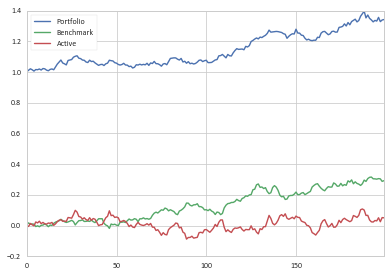
Now we see that the active return plus the benchmark return plus the initial cash equals the current value of the portfolio.

   >>> df_cum.tail(3)[['Benchmark', 'Active', 'Portfolio']]
         Benchmark    Active  Portfolio
    197   0.303995  0.024725   1.328720
    198   0.287709  0.051606   1.339315
    199   0.292082  0.050098   1.342179

By construction, df_cum['Portfolio'] = 1 + df_cum['Benchmark'] + df_cum['Active']. Because this method is difficult to calculate (without Pandas!) and understand (most people won't get the notional exposures), industry practice generally defines the active return as the cumulative difference in returns over a period of time. For example, if a fund was up 5.0% in a month and the market was down 1.0%, then the excess return for that month is generally defined as +6.0%. The problem with this simplistic approach, however, is that your results will drift apart over time due to compounding and rebalancing issues that aren't properly factored into the calculations.

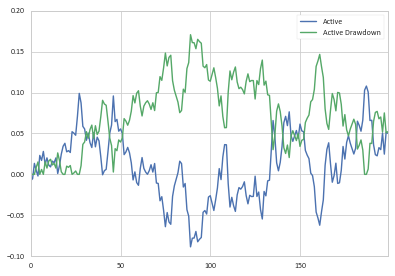
So given our df_cum.Active column, we could define the drawdown as:

drawdown = pd.Series(1 - (1 + df_cum.Active)/(1 + df_cum.Active.cummax()), name='Active Drawdown')

>>> df_cum.Active.plot(legend=True);drawdown.plot(legend=True)

You can then determine the start and end points of the drawdown as you have previously done.

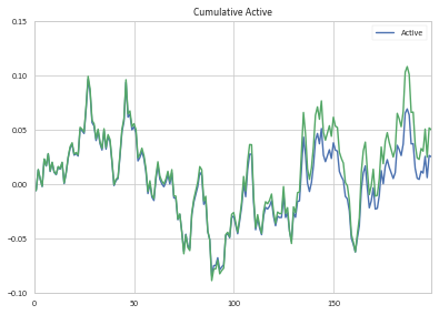
Comparing my cumulative Active return contribution with the amounts you calculated, you will find them to be similar at first, and then drift apart over time (my return calcs are in green):

Luci

You have uncovered that I calculated cumulative active return incorrectly. I intended to cumulate the 'Portfolio' and 'Benchmark' returns prior to taking the difference. Instead, I took the difference in period returns and cumulated them. This is a mistake, as you've highlighted. I've corrected that calculation. Fortunately, it does not impact the calculation of the max_active_drawdown as it was an error in the demonstration. Thanks for catching that. – Hypogastrium

Answer 3

My cheap two pennies in pure Python:

def find_drawdown(lista):
    peak = 0
    trough = 0
    drawdown = 0
    for n in lista:
        if n > peak:
            peak = n
            trough = peak
        if n < trough:
            trough = n
        temp_dd = peak - trough
        if temp_dd > drawdown:
            drawdown = temp_dd
    return -drawdown

Epitasis

Answer 4

In piRSquared answer I would suggest amending

pmb = p - b 

to

pmb = p / b 

to find the rel. maxDD. df3 using pmb = p-b identifies a rel. MaxDD of US$851 (-48.9%). df2 using pmb = p/b identifies the rel. MaxDD as US$544.6 (-57.9%)

import pandas as pd
import datetime
import pandas_datareader.data as pdr
import matplotlib.pyplot as plt
import yfinance as yfin
yfin.pdr_override()
stocks = ["AMZN", "SPY"]
df = pdr.get_data_yahoo(stocks, start="2020-01-01", end="2022-02-18")
df = df[['Adj Close']]
df.columns = df.columns.droplevel(0)
df.reset_index(inplace=True)
df.Date=df.Date.dt.date

df2 = df[df.Date.isin([datetime.date(2020,7,9), datetime.date(2022,2,3)])].copy()
df2['AMZN/SPY'] = df2.AMZN / df2.SPY
df2['AMZN-SPY'] = df2.AMZN - df2.SPY
df2['USDdiff'] = df2['AMZN-SPY'].diff().round(1)
df2[["p", "b"]] = df2[['AMZN','SPY']].pct_change(1).round(4)
df2['p-b'] = df2.p - df2.b
df2.replace(np. nan,'',regex=True, inplace=True)
df2 = df2.round(2)
print(df2)


      Date     AMZN    SPY  AMZN/SPY  AMZN-SPY USDdiff       p       b      p-b
2020-07-09  3182.63  307.7     10.34   2874.93                           
2022-02-03  2776.91  446.6      6.22   2330.31  -544.6 -0.1275  0.4514  -0.5789 

   
df3 = df[df.Date.isin([datetime.date(2020,9,2), datetime.date(2022,2,3)])].copy()
df3['AMZN/SPY'] = df3.AMZN / df3.SPY
df3['AMZN-SPY'] = df3.AMZN - df3.SPY
df3['USDdiff'] = df3['AMZN-SPY'].diff().round(1)
df3[["p", "b"]] = df3[['AMZN','SPY']].pct_change(1).round(4)
df3['p-b'] = df3.p - df3.b
df3.replace(np. nan,'',regex=True, inplace=True)
df3 = df3.round(2)
print(df3)
    
      Date     AMZN     SPY  AMZN/SPY  AMZN-SPY USDdiff       p       b      p-b 
2020-09-02  3531.45  350.09     10.09   3181.36                           
2022-02-03  2776.91  446.60      6.22   2330.31  -851.0 -0.2137  0.2757  -0.4894   

   

PS: I don't have enough reputation to comment.

Appetence