Calculate max draw down with a vectorized solution in python
Asked Answered
H

4

17

Maximum Drawdown is a common risk metric used in quantitative finance to assess the largest negative return that has been experienced.

Recently, I became impatient with the time to calculate max drawdown using my looped approach.

def max_dd_loop(returns):
    """returns is assumed to be a pandas series"""
    max_so_far = None
    start, end = None, None
    r = returns.add(1).cumprod()
    for r_start in r.index:
        for r_end in r.index:
            if r_start < r_end:
                current = r.ix[r_end] / r.ix[r_start] - 1
                if (max_so_far is None) or (current < max_so_far):
                    max_so_far = current
                    start, end = r_start, r_end
    return max_so_far, start, end

I'm familiar with the common perception that a vectorized solution would be better.

The questions are:

  • can I vectorize this problem?
  • What does this solution look like?
  • How beneficial is it?

Edit

I modified Alexander's answer into the following function:

def max_dd(returns):
    """Assumes returns is a pandas Series"""
    r = returns.add(1).cumprod()
    dd = r.div(r.cummax()).sub(1)
    mdd = dd.min()
    end = dd.argmin()
    start = r.loc[:end].argmax()
    return mdd, start, end
Handbarrow answered 20/4, 2016 at 17:4 Comment(6)
See if this question and answer provide any help: #21058833Imprison
See also #22607824 (possibly a duplicate?)Imprison
Way late to the game, but I think r.loc[:end].argmax() will give you an issue here. You want r.loc[:end].sort_index(ascending=False).argmax(). If you have multiple zeros in your Series (multiple high water marks), the current line as-is will return the first rather than last occurrence and yield a start date that's way too early.Bordereau
@BradSolomon unless I'm missing something, If there are multiple and identical high water marks, it's a matter of interpretation as to when the period of maximum drawdown occurred. Further, this doesn't effect the calculation of the return.Handbarrow
Say you have a drawdown Series (not a return Series) [0, 0, -2, 0, -3, -5] indexed by the first 6 months of the year. The high water mark before the -5 drawdown period is the third 0 (April), not the first, so not using .sort_index(ascending=False) to reverse the Series would incorrectly tell you your drawdown started in Jan. I guess it's interpretation, but under that method wouldn't every drawdown start at month 0 or month 1? I've never seen the start date described as such. The HWMs don't have to be identical to get multiple zeros in your drawdown series.Bordereau
@Handbarrow The functions argmin & argmax are deprecated now... FutureWarning: 'argmax' is deprecated. Use 'idxmax' instead. The behavior of 'argmax' will be corrected to return the positional maximum in the future. Use 'series.values.argmax' to get the position of the maximum now. How did you solve this?Rebuke
N
24

df_returns is assumed to be a dataframe of returns, where each column is a seperate strategy/manager/security, and each row is a new date (e.g. monthly or daily).

cum_returns = (1 + df_returns).cumprod()
drawdown =  1 - cum_returns.div(cum_returns.cummax())
Neelon answered 20/4, 2016 at 17:13 Comment(3)
Thanks Alexander! This is much faster than the answer I gave. I was oblivious to the cummax() method. I have to modify the code a bit to return the start and end points but this is what I wanted.Handbarrow
This does not correctly take into account the first return in the series. The high water mark in this example should be 1 not 0.9. df_returns = pd.Series([-.1,-.1,-.1,-.1]) cum_returns = (1 + df_returns).cumprod() drawdown = 1 - cum_returns.div(cum_returns.cummax()) ) print(cum_returns.cummax()) print(drawdown.max()) 0 0.9 1 0.9 2 0.9 3 0.9 4 0.9 dtype: float64 0.18999999999999995Delldella
@Delldella Your observation appears to be correct. One would need to include a return of zero on the initial investment date, e.g. df_returns = pd.concat([pd.Series(0, index=[{initial_investment_date}]), df_returns]). This may have been assumed in the initial question, but there is no sample data so one cannot be sure.Neelon
B
4

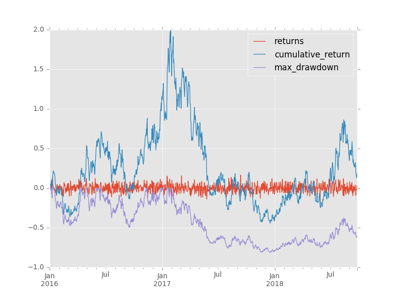
I had first suggested using .expanding() window but that's obviously not necessary with the .cumprod() and .cummax() built ins to calculate max drawdown up to any given point:

df = pd.DataFrame(data={'returns': np.random.normal(0.001, 0.05, 1000)}, index=pd.date_range(start=date(2016,1,1), periods=1000, freq='D'))

df = pd.DataFrame(data={'returns': np.random.normal(0.001, 0.05, 1000)},
                  index=pd.date_range(start=date(2016, 1, 1), periods=1000, freq='D'))
df['cumulative_return'] = df.returns.add(1).cumprod().subtract(1)
df['max_drawdown'] = df.cumulative_return.add(1).div(df.cumulative_return.cummax().add(1)).subtract(1)

enter image description here

            returns  cumulative_return  max_drawdown
2016-01-01 -0.014522          -0.014522      0.000000
2016-01-02 -0.022769          -0.036960     -0.022769
2016-01-03  0.026735          -0.011214      0.000000
2016-01-04  0.054129           0.042308      0.000000
2016-01-05 -0.017562           0.024004     -0.017562
2016-01-06  0.055254           0.080584      0.000000
2016-01-07  0.023135           0.105583      0.000000
2016-01-08 -0.072624           0.025291     -0.072624
2016-01-09 -0.055799          -0.031919     -0.124371
2016-01-10  0.129059           0.093020     -0.011363
2016-01-11  0.056123           0.154364      0.000000
2016-01-12  0.028213           0.186932      0.000000
2016-01-13  0.026914           0.218878      0.000000
2016-01-14 -0.009160           0.207713     -0.009160
2016-01-15 -0.017245           0.186886     -0.026247
2016-01-16  0.003357           0.190869     -0.022979
2016-01-17 -0.009284           0.179813     -0.032050
2016-01-18 -0.027361           0.147533     -0.058533
2016-01-19 -0.058118           0.080841     -0.113250
2016-01-20 -0.049893           0.026914     -0.157492
2016-01-21 -0.013382           0.013173     -0.168766
2016-01-22 -0.020350          -0.007445     -0.185681
2016-01-23 -0.085842          -0.092648     -0.255584
2016-01-24  0.022406          -0.072318     -0.238905
2016-01-25  0.044079          -0.031426     -0.205356
2016-01-26  0.045782           0.012917     -0.168976
2016-01-27 -0.018443          -0.005764     -0.184302
2016-01-28  0.021461           0.015573     -0.166797
2016-01-29 -0.062436          -0.047836     -0.218819
2016-01-30 -0.013274          -0.060475     -0.229189
...              ...                ...           ...
2018-08-28  0.002124           0.559122     -0.478738
2018-08-29 -0.080303           0.433921     -0.520597
2018-08-30 -0.009798           0.419871     -0.525294
2018-08-31 -0.050365           0.348359     -0.549203
2018-09-01  0.080299           0.456631     -0.513004
2018-09-02  0.013601           0.476443     -0.506381
2018-09-03 -0.009678           0.462153     -0.511158
2018-09-04 -0.026805           0.422960     -0.524262
2018-09-05  0.040832           0.481062     -0.504836
2018-09-06 -0.035492           0.428496     -0.522411
2018-09-07 -0.011206           0.412489     -0.527762
2018-09-08  0.069765           0.511031     -0.494817
2018-09-09  0.049546           0.585896     -0.469787
2018-09-10 -0.060201           0.490423     -0.501707
2018-09-11 -0.018913           0.462235     -0.511131
2018-09-12 -0.094803           0.323611     -0.557477
2018-09-13  0.025736           0.357675     -0.546088
2018-09-14 -0.049468           0.290514     -0.568542
2018-09-15  0.018146           0.313932     -0.560713
2018-09-16 -0.034118           0.269104     -0.575700
2018-09-17  0.012191           0.284576     -0.570527
2018-09-18 -0.014888           0.265451     -0.576921
2018-09-19  0.041180           0.317562     -0.559499
2018-09-20  0.001988           0.320182     -0.558623
2018-09-21 -0.092268           0.198372     -0.599348
2018-09-22 -0.015386           0.179933     -0.605513
2018-09-23 -0.021231           0.154883     -0.613888
2018-09-24 -0.023536           0.127701     -0.622976
2018-09-25  0.030160           0.161712     -0.611605
2018-09-26  0.025528           0.191368     -0.601690
Bucentaur answered 20/4, 2016 at 17:36 Comment(0)
H
2

Given a time series of returns, we need to evaluate the aggregate return for every combination of starting point to ending point.

The first trick is to convert a time series of returns into a series of return indices. Given a series of return indices, I can calculate the return over any sub-period with the return index at the beginning ri_0 and at the end ri_1. The calculation is: ri_1 / ri_0 - 1.

The second trick is to produce a second series of inverses of return indices. If r is my series of return indices then 1 / r is my series of inverses.

The third trick is to take the matrix product of r * (1 / r).Transpose.

r is an n x 1 matrix. (1 / r).Transpose is a 1 x n matrix. The resulting product contains every combination of ri_j / ri_k. Just subtract 1 and I've actually got returns.

The fourth trick is to ensure that I'm constraining my denominator to represent periods prior to those being represented by the numerator.

Below is my vectorized function.

import numpy as np
import pandas as pd

def max_dd(returns):
    # make into a DataFrame so that it is a 2-dimensional
    # matrix such that I can perform an nx1 by 1xn matrix
    # multiplication and end up with an nxn matrix
    r = pd.DataFrame(returns).add(1).cumprod()

    # I copy r.T to ensure r's index is not the same
    # object as 1 / r.T's columns object
    x = r.dot(1 / r.T.copy()) - 1
    x.columns.name, x.index.name = 'start', 'end'

    # let's make sure we only calculate a return when start
    # is less than end.
    y = x.stack().reset_index()
    y = y[y.start < y.end]

    # my choice is to return the periods and the actual max
    # draw down
    z = y.set_index(['start', 'end']).iloc[:, 0]
    return z.min(), z.argmin()[0], z.argmin()[1]

How does this perform?

for the vectorized solution I ran 10 iterations over the time series of lengths [10, 50, 100, 150, 200]. The time it took is below:

10:   0.032 seconds
50:   0.044 seconds
100:  0.055 seconds
150:  0.082 seconds
200:  0.047 seconds

The same test for the looped solution is below:

10:   0.153 seconds
50:   3.169 seconds
100: 12.355 seconds
150: 27.756 seconds
200: 49.726 seconds

Edit

Alexander's answer provides superior results. Same test using modified code

10:   0.000 seconds
50:   0.000 seconds
100:  0.004 seconds
150:  0.007 seconds
200:  0.008 seconds

I modified his code into the following function:

def max_dd(returns):
    r = returns.add(1).cumprod()
    dd = r.div(r.cummax()).sub(1)
    mdd = drawdown.min()
    end = drawdown.argmin()
    start = r.loc[:end].argmax()
    return mdd, start, end
Handbarrow answered 20/4, 2016 at 17:4 Comment(0)
U
0

I recently had a similar issue, but instead of a global MDD, I was required to find the MDD for the interval after each peak. Also, in my case, I was supposed to take the MDD of each strategy alone and thus wasn't required to apply the cumprod. My vectorized implementation is also based on Investopedia.

def calc_MDD(networth):
  df = pd.Series(networth, name="nw").to_frame()

  max_peaks_idx = df.nw.expanding(min_periods=1).apply(lambda x: x.argmax()).fillna(0).astype(int)
  df['max_peaks_idx'] = pd.Series(max_peaks_idx).to_frame()

  nw_peaks = pd.Series(df.nw.iloc[max_peaks_idx.values].values, index=df.nw.index)

  df['dd'] = ((df.nw-nw_peaks)/nw_peaks)
  df['mdd'] = df.groupby('max_peaks_idx').dd.apply(lambda x: x.expanding(min_periods=1).apply(lambda y: y.min())).fillna(0)

  return df

Here is an sample after running this code:

        nw      max_peaks_idx       dd          mdd
0   10000.000       0           0.000000    0.000000
1   9696.948        0           -0.030305   -0.030305
2   9538.576        0           -0.046142   -0.046142
3   9303.953        0           -0.069605   -0.069605
4   9247.259        0           -0.075274   -0.075274
5   9421.519        0           -0.057848   -0.075274
6   9315.938        0           -0.068406   -0.075274
7   9235.775        0           -0.076423   -0.076423
8   9091.121        0           -0.090888   -0.090888
9   9033.532        0           -0.096647   -0.096647
10  8947.504        0           -0.105250   -0.105250
11  8841.551        0           -0.115845   -0.115845

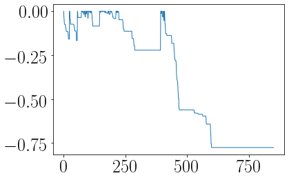
And here is an image of the complete applied to the complete dataset.

enter image description here

Although vectorized, this code is probably slower than the other, because for each time-series, there should be many peaks, and each one of these requires calculation, and so O(n_peaks*n_intervals).

PS: I could have eliminated the zero values in the dd and mdd columns, but I find it useful that these values help indicate when a new peak was observed in the time-series.

Unilobed answered 18/4, 2020 at 19:30 Comment(0)

© 2022 - 2024 — McMap. All rights reserved.