Confidence interval for exponential curve fit

Question

I'm trying to obtain a confidence interval on an exponential fit to some x,y data (available here). Here's the MWE I have to find the best exponential fit to the data:

from pylab import *
from scipy.optimize import curve_fit

# Read data.
x, y = np.loadtxt('exponential_data.dat', unpack=True)

def func(x, a, b, c):
    '''Exponential 3-param function.'''
    return a * np.exp(b * x) + c

# Find best fit.
popt, pcov = curve_fit(func, x, y)
print popt

# Plot data and best fit curve.
scatter(x, y)
x = linspace(11, 23, 100)
plot(x, func(x, *popt), c='r')
show()

which produces:

How can I obtain the 95% (or some other value) confidence interval on this fit preferably using either pure python, numpy or scipy (which are the packages I already have installed)?

Quell

https://mcmap.net/q/302463/-show-confidence-limits-and-prediction-limits-in-scatter-plot – Homogenize

Answer 1

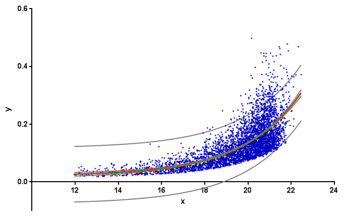
Gabriel's answer is incorrect. Here in red the 95% confidence band for his data as calculated by GraphPad Prism:

Background: the "confidence interval of a fitted curve" is typically called confidence band. For a 95% confidence band, one can be 95% confident that it contains the true curve. (This is different from prediction bands, shown above in gray. Prediction bands are about future data points. For more details, see, e.g., this page of the GraphPad Curve Fitting Guide.)

In Python, kmpfit can calculate the confidence band for non-linear least squares. Here for Gabriel's example:

from pylab import *
from kapteyn import kmpfit

x, y = np.loadtxt('_exp_fit.txt', unpack=True)

def model(p, x):
  a, b, c = p
  return a*np.exp(b*x)+c

f = kmpfit.simplefit(model, [.1, .1, .1], x, y)
print f.params

# confidence band
a, b, c = f.params
dfdp = [np.exp(b*x), a*x*np.exp(b*x), 1]
yhat, upper, lower = f.confidence_band(x, dfdp, 0.95, model)

scatter(x, y, marker='.', s=10, color='#0000ba')
ix = np.argsort(x)
for i, l in enumerate((upper, lower, yhat)):
  plot(x[ix], l[ix], c='g' if i == 2 else 'r', lw=2)
show()

The dfdp are the partial derivatives ∂f/∂p of the model f = a*e^(b*x) + c with respect to each parameter p (i.e., a, b, and c). For background, see the kmpfit Tutorial or this page of the GraphPad Curve Fitting Guide. (Unlike my sample code, the kmpfit Tutorial does not use confidence_band() from the library but its own, slightly different, implementation.)

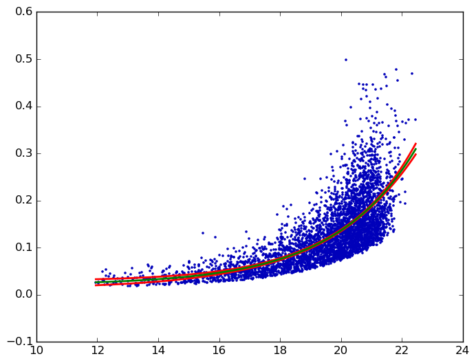
Finally, the Python plot matches the Prism one:

Convexoconcave

Great answer Ulrich, thank you very much! Indeed, I believe my old answer actually obtains the prediction bands rather than the fitted curve's confidence interval. You seem to know your way around these stats, could you confirm this is the case? – Quell

I just added prediction bands to the Prism plot. So your old answer does not calculate prediction bands. This page of the GraphPad Curve Fitting Guide states how they are calculated in Prism. – Convexoconcave

Answer 2

You can use the uncertainties module to do the uncertainty calculations. uncertainties keeps track of uncertainties and correlation. You can create correlated uncertainties.ufloat directly from the output of curve_fit.

To be able to do those calculation on non-builtin operations such as exp you need to use the functions from uncertainties.unumpy.

You should also avoid your from pylab import * import. This even overwrites python built-ins such as sum.

A complete example:

import numpy as np
from scipy.optimize import curve_fit
import uncertainties as unc
import matplotlib.pyplot as plt
import uncertainties.unumpy as unp


def func(x, a, b, c):
    '''Exponential 3-param function.'''
    return a * np.exp(b * x) + c

x, y = np.genfromtxt('data.txt', unpack=True)

popt, pcov = curve_fit(func, x, y)

a, b, c = unc.correlated_values(popt, pcov)

# Plot data and best fit curve.
plt.scatter(x, y, s=3, linewidth=0, alpha=0.3)

px = np.linspace(11, 23, 100)
# use unumpy.exp
py = a * unp.exp(b * px) + c

nom = unp.nominal_values(py)
std = unp.std_devs(py)

# plot the nominal value
plt.plot(px, nom, c='r')

# And the 2sigma uncertaintie lines
plt.plot(px, nom - 2 * std, c='c')
plt.plot(px, nom + 2 * std, c='c')
plt.savefig('fit.png', dpi=300)

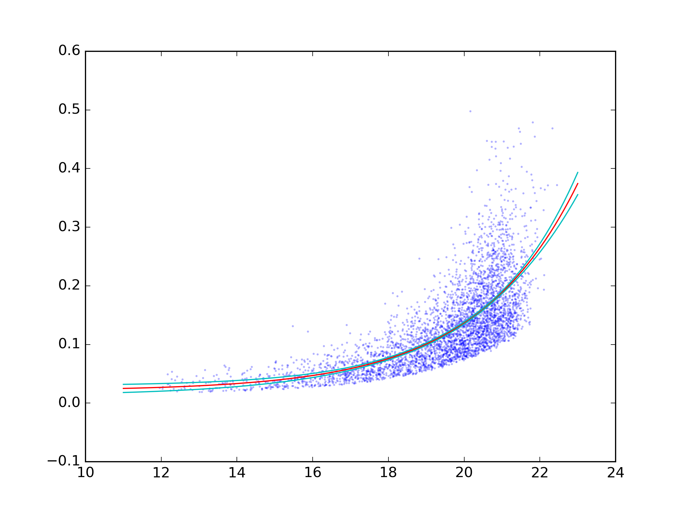
And the result:

Mcmahon

I wasn't aware of the uncertainties package, I'll give it a try it looks very interesting. Thank you very much! – Quell

Oh man, I did not even know that I was looking for it all the years. – Leclaire

Answer 3

Notice: the actual answer to obtaining the fitted curve's confidence interval is given by Ulrich here.

---

After some research (see here, here and 1.96) I came up with my own solution.

It accepts an arbitrary X% confidence interval and plots upper and lower curves.

Here's the MWE:

from pylab import *
from scipy.optimize import curve_fit
from scipy import stats


def func(x, a, b, c):
    '''Exponential 3-param function.'''
    return a * np.exp(b * x) + c


# Read data.
x, y = np.loadtxt('exponential_data.dat', unpack=True)

# Define confidence interval.
ci = 0.95
# Convert to percentile point of the normal distribution.
# See: https://en.wikipedia.org/wiki/Standard_score
pp = (1. + ci) / 2.
# Convert to number of standard deviations.
nstd = stats.norm.ppf(pp)
print nstd

# Find best fit.
popt, pcov = curve_fit(func, x, y)
# Standard deviation errors on the parameters.
perr = np.sqrt(np.diag(pcov))
# Add nstd standard deviations to parameters to obtain the upper confidence
# interval.
popt_up = popt + nstd * perr
popt_dw = popt - nstd * perr

# Plot data and best fit curve.
scatter(x, y)
x = linspace(11, 23, 100)
plot(x, func(x, *popt), c='g', lw=2.)
plot(x, func(x, *popt_up), c='r', lw=2.)
plot(x, func(x, *popt_dw), c='r', lw=2.)
text(12, 0.5, '{}% confidence interval'.format(ci * 100.))    

show()

Quell

when you already have x,y from exponential_data.dat why do you again say x = linspace(11,23,100). It would be better to call it X1 or something so that people dont get confused. I can understand that it is for the confidence lines. – Copenhagen

I also found out another solution. The covariance matrix pcov in our curve_fit has the 1sigma error which can be used as well. Check this WEBSITE – Copenhagen

@ThePredator because if I'd called the full x instead of linspace(11,23,100) the function would try to plot the fitted curve to touch all those x values. Try it for yourself commenting out x = linspace(11, 23, 100) and see what happens :) – Quell

@ThePredator The covariance matrix pcov is exactly what my answer uses: perr = np.sqrt(np.diag(pcov)). Those are the 1 sigma errors, that's how you obtain them (see here) – Quell

I don't think that this solution is correct. I see two major problems here: (1) Choosing the margin of one parameters confidence interval gets you to 95%, taking the also the second gets you to 1-0.05**2 --> 99.75%. So your confidence interval here is way bigger. (2) You assume your parameters to be independent, what is an legit approximation only when your co-variances are small. – Killifish

Answer 4

curve_fit() returns the covariance matrix - pcov -- which holds the estimated uncertainties (1 sigma). This assumes errors are normally distributed, which is sometimes questionable.

You might also consider using the lmfit package (pure python, built on top of scipy), which provides a wrapper around scipy.optimize fitting routines (including leastsq(), which is what curve_fit() uses) and can, among other things, calculate confidence intervals explicitly.

Crowfoot

Answer 5

I've always been a fan of simple bootstrapping to get confidence intervals. If you have n data points, then use the random package to select n points from your data WITH RESAMPLING (i.e. allow your program to get the same point multiple times if that's what it wants to do - very important). Once you've done that, plot the resampled points and get the best fit. Do this 10,000 times, getting a new fit line each time. Then your 95% confidence interval is the pair of lines that enclose 95% of the best fit lines you made.

It's a pretty easy method to program in Python, but it's a bit unclear how this would work out from a statistical point of view. Some more information on why you want to do this would probably lead to more appropriate answers for your task.

Norean