What is C parameter in sklearn Logistic Regression?

Question

What is the meaning of C parameter in sklearn.linear_model.LogisticRegression? How does it affect the decision boundary? Do high values of C make the decision boundary non-linear? How does overfitting look like for logistic regression if we visualize the decision boundary?

Barbwire

Does this answer your question? What is the inverse of regularization strength in Logistic Regression? How should it affect my code? – Benedetta

It answers only the first part of the question (What is the meaning of C parameter). I care about the visualization part (i.e. how does it affect the shape of the decision boundary). I hoped someone would provide an example with visualization. – Barbwire

I can imagine how overfitting looks like for nonlinear decision boundaries (squiggly line), but for linear models such as logistic regression how can we imagine the shape of decision boundary using different C values? – Barbwire

Answer 1

From the documentation:

C: float, default=1.0 Inverse of regularization strength; must be a positive float. Like in support vector machines, smaller values specify stronger regularization.

If you don't understand that, Cross Validated may be a better place to ask than here.

While CS people will often refer to all the arguments to a function as "parameters", in machine learning, C is referred to as a "hyperparameter". The parameters are numbers that tells the model what to do with the features, while hyperparameters tell the model how to choose parameters.

Regularization generally refers the concept that there should be a complexity penalty for more extreme parameters. The idea is that just looking at the training data and not paying attention to how extreme one's parameters are leads to overfitting. A high value of C tells the model to give high weight to the training data, and a lower weight to the complexity penalty. A low value tells the model to give more weight to this complexity penalty at the expense of fitting to the training data. Basically, a high C means "Trust this training data a lot", while a low value says "This data may not be fully representative of the real world data, so if it's telling you to make a parameter really large, don't listen to it".

https://en.wikipedia.org/wiki/Regularization_(mathematics)

Lapides

Please can you provide an example of the difference in decision boundary between low and high C values? As far as I know, logistic regression always has a linear decision boundary, so how does it have like a flexible decision boundary for large C values? – Barbwire

Answer 2

What is regularization?

Logistic Regression is an optimization problem that minimizes a cost function. Regularization adds a penalty term to this cost function, so essentially it changes the objective function and the problem becomes different from the one without a penalty term. The penalty term consists of the coefficients of the model and adding it penalizes large coefficients (because large coefficients would increase the value of the objective function that is being minimized) and "artificially" makes them smaller.

Regularization helps if the model is overfit (a classic example is it has too many variables). If it's not overfit, there is no need for regularization. A graph further down this post will show the difference.

An easy way to code the internal optimization is via a log-likelihood function (logistic regression maximizes log-likelihood). A two-line code that does that is as follows.

scores = X.dot(coefficients) + intercept
log_likelihood = np.sum((y-1)*scores - np.log(1 + np.exp(-scores)))

Regularization adds a penalty term, so now, the log-likelihood would look like:

penalty_term = (1 / C if C else 0) * np.sum(coefficients**2)   # only regularize non-intercept coefficients
log_likelihood = np.sum((y-1)*scores - np.log(1 + np.exp(-scores))) - penalty_term
#                                                                   ^^^^^^^^^^^^^^  <--- penalty here

If we were to write a logistic regression from scratch, it would simply be a loop where in each step, the coefficients are updated so that the error becomes smaller and smaller.

from sklearn.datasets import make_classification
import numpy as np

def logistic_regression(X, y, C=None, step_size=0.005):
    
    coef_ = np.array([0.]*X.shape[1])
    l2_penalty = 1 / C if C else 0
    
    for ctr in range(100):
        # predict P(y_i = 1 | X_i, coef_)
        predicted_proba = 1 / (1 + np.exp(-X.dot(coef_)))
        errors = y - predicted_proba
        # add penalty only for non-intercept 
        penalty = 2*l2_penalty*coef_*[0, *[1]*(len(coef_)-1)]
        # compute derivatives and add penalty
        derivatives = X.T.dot(errors) - penalty
        # update the coefficients
        coef_ += step_size * derivatives
        
    return coef_

def log_likelihood(X, y, coef_, C=None):
    penalty_term = (1 / C if C else 0) * np.sum(coef_[1:]**2)
    scores = X.dot(coef_)
    return np.sum((y-1)*scores - np.log(1 + np.exp(-scores))) - penalty_term

def compute_accuracy(X, y, coef_):
    predictions = (X.dot(coef_) > 0)
    return np.mean(predictions == y)


# example
X, y = make_classification()
X_ = np.c_[[1]*100, X]
coefs = logistic_regression(X_, y, C=0.01)
accuracy = compute_accuracy(X_, y, coefs)

scikit-learn's LogisticRegression regularizes by default(?!)

If we circle back to scikit-learn, as mentioned earlier, because coefficients become smaller with regularization, it is important to scale the data fed into the model (perhaps with StandardScaler()) because the magnitude of the coefficients depend on the variable scale. However, scikit-learn's LogisticRegression is, inexplicably, regularized by default (C: float, default=1.0 as documented) and you have to actually actually set penalty=None to solve for the non-regularized coefficients.

Decision boundaries of not overfit vs overfit models

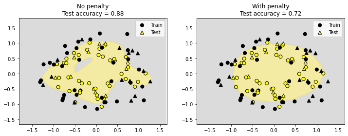
As mentioned earlier, if the model is not overfit, there is no need for regularization (so with scikit-learn, penalty=None should be set). The graph below shows the class regions (using a contour plot) for two trained models (one without regularization and one with regularization). The one without regularization performs better on test data which is also confirmed by the class regions plotted.

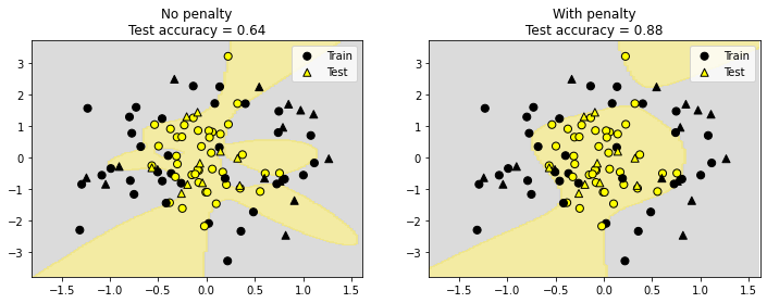
Now, if the model is overfit (the class regions without regularization looks pretty ridiculous and fits a lot of the training data noise), regularization is useful, as confirmed by the test accuracy of the model with regularization.

---

Code used to produce the contour plots.

import numpy as np
import matplotlib.pyplot as plt
from sklearn.datasets import make_circles
from sklearn.model_selection import train_test_split
from sklearn.preprocessing import PolynomialFeatures
from sklearn.linear_model import LogisticRegression
from matplotlib.colors import ListedColormap

def plot_class_regions(clf, transformer, X, y, ax=None):

    if ax is None:
        fig, ax = plt.subplots(figsize=(6,6))
    
    # lighter cmap for contour filling and darker cmap for markers
    cmap_light = ListedColormap(['lightgray', 'khaki'])
    cmap_bold  = ListedColormap(['black', 'yellow'])

    # create a sample for contour plot
    x_min, x_max = X[:, 0].min()-0.5, X[:, 0].max()+0.5
    y_min, y_max = X[:, 1].min()-0.5, X[:, 1].max()+0.5
    x2, y2 = np.meshgrid(np.arange(x_min, x_max, 0.03), np.arange(y_min, y_max, 0.03))
    
    # transform sample
    sample = np.c_[x2.ravel(), y2.ravel()]
    if transformer:
        sample = transformer.transform(sample)
        
    # make predictions
    preds = clf.predict(sample).reshape(x2.shape)
    # plot contour
    ax.contourf(x2, y2, preds, cmap=cmap_light, alpha=0.8)
    # scatter plot
    ax.scatter(X[:, 0], X[:, 1], c=y, cmap=cmap_bold, s=50, edgecolor='black', label='Train')
    ax.set(xlim=(x_min, x_max), ylim=(y_min, y_max))
    
    return ax

def plotter(X, y):
    
    # train-test-split
    X_train, X_test, y_train, y_test = train_test_split(X, y, random_state=0)
    # add more features
    poly = PolynomialFeatures(degree=6)
    X_poly = poly.fit_transform(X_train)

    fig, axs = plt.subplots(1, 2, figsize=(12,4), facecolor='white')

    for i, lr in enumerate([LogisticRegression(penalty=None, max_iter=10000), 
                            LogisticRegression(max_iter=2000)]):
        
        lr.fit(X_poly, y_train)

        plot_class_regions(lr, poly, X_train, y_train, axs[i])
        axs[i].scatter(X_test[:, 0], X_test[:, 1], c=y_test, cmap=ListedColormap(['black', 'yellow']), 
                   s=50, marker='^', edgecolor='black', label='Test')
        axs[i].set_title(f"{'No' if i == 0 else 'With'} penalty\nTest accuracy = {lr.score(poly.transform(X_test), y_test)}")
        axs[i].legend()
        
# not overfit -- no need for regularization
X, y = make_circles(factor=0.7, noise=0.2, random_state=2023)
plotter(X, y)

# overfit -- needs regularization
X, y = make_circles(factor=0.3, noise=0.2, random_state=2023)
X[:, 1] += np.random.default_rng(2023).normal(size=len(X))
plotter(X, y)

Bushmaster