Let's have a look at the source code:
In the filter_update function pykalman checks, if the current observation is masked or not.
def filter_update(...)

        # Make a masked observation if necessary
        if observation is None:
            n_dim_obs = observation_covariance.shape[0]
            observation = np.ma.array(np.zeros(n_dim_obs))
            observation.mask = True
        else:
            observation = np.ma.asarray(observation)
It does not impact the prediction step. But the correction step have two options. It happens in the _filter_correct function.
def _filter_correct(...)

    if not np.any(np.ma.getmask(observation)):

         # the normal Kalman Filter math

    else:
        n_dim_state = predicted_state_covariance.shape[0]
        n_dim_obs = observation_matrix.shape[0]
        kalman_gain = np.zeros((n_dim_state, n_dim_obs))

        # !!!! the corrected state takes the result of the prediction !!!!

        corrected_state_mean = predicted_state_mean
        corrected_state_covariance = predicted_state_covariance
So as you can see this is exactly the theoretical approach.
Here is a short example and working data to play with.
Assume you have a gps receiver and you want to track yourself while walking. The receiver has a good accuracy. For simplification assume you go straight forward only.
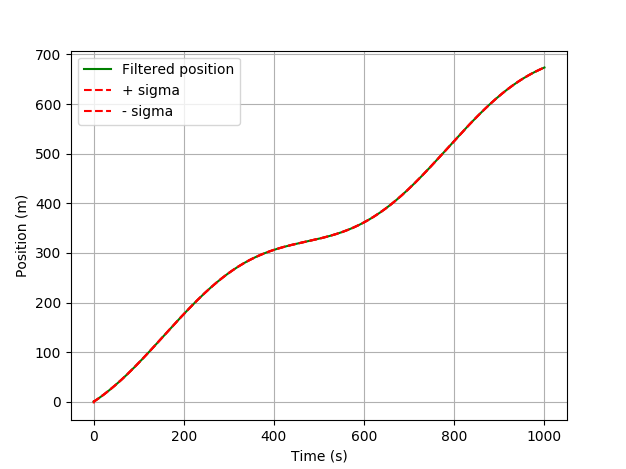
![pykalman estimation of the position using a gps receiver without masked observations]()
Nothing interesting happens. The filter estimates your position very well because of a good gps signal. What happens if you have no signal for a while?
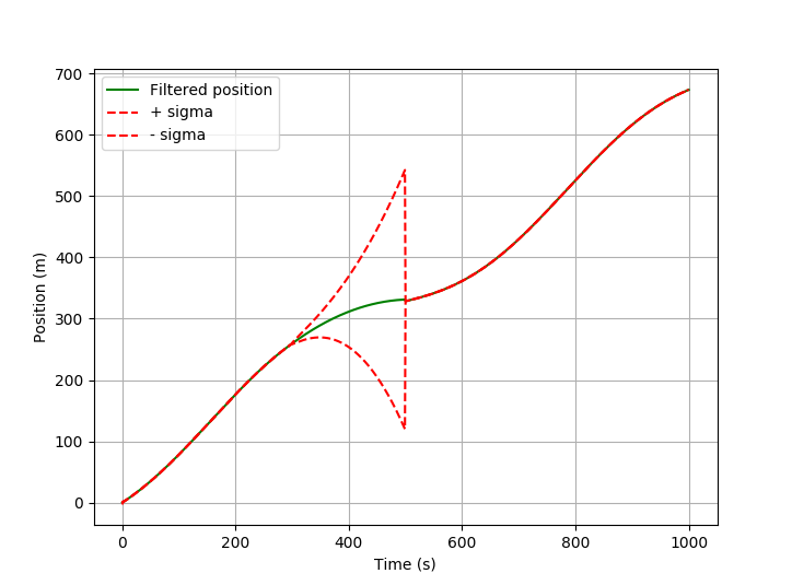
![pykalman estimation using masked observations]()
The filter can only predict based on the existing state and the knowledge about the system dynamics (see matrix Q). With each prediction step the uncertainty grows. The 1-Sigma range around the estimated position gets bigger. As soon as a new observation is there again, the state is corrected.
Here is the code and the data:
from pykalman import KalmanFilter
import numpy as np
import matplotlib.pyplot as plt
from numpy import ma

# enable or disable missing observations
use_mask = 1

# reading data (quick and dirty)
Time=[]
X=[]

for line in open('data/dataset_01.csv'):
    f1, f2  = line.split(';')
    Time.append(float(f1))
    X.append(float(f2))

if (use_mask):
    X = ma.asarray(X)
    X[300:500] = ma.masked

# Filter Configuration

# time step
dt = Time[2] - Time[1]

# transition_matrix
F = [[1,  dt,   0.5*dt*dt],
     [0,   1,          dt],
     [0,   0,           1]]

# observation_matrix
H = [1, 0, 0]

# transition_covariance
Q = [[   1,     0,     0],
     [   0,  1e-4,     0],
     [   0,     0,  1e-6]]

# observation_covariance
R = [0.04] # max error = 0.6m

# initial_state_mean
X0 = [0,
      0,
      0]

# initial_state_covariance
P0 = [[ 10,    0,   0],
      [  0,    1,   0],
      [  0,    0,   1]]

n_timesteps = len(Time)
n_dim_state = 3

filtered_state_means = np.zeros((n_timesteps, n_dim_state))
filtered_state_covariances = np.zeros((n_timesteps, n_dim_state, n_dim_state))

# Kalman-Filter initialization
kf = KalmanFilter(transition_matrices = F,
                  observation_matrices = H,
                  transition_covariance = Q,
                  observation_covariance = R,
                  initial_state_mean = X0,
                  initial_state_covariance = P0)


# iterative estimation for each new measurement
for t in range(n_timesteps):
    if t == 0:
        filtered_state_means[t] = X0
        filtered_state_covariances[t] = P0
    else:
        filtered_state_means[t], filtered_state_covariances[t] = (
        kf.filter_update(
            filtered_state_means[t-1],
            filtered_state_covariances[t-1],
            observation = X[t])
        )

position_sigma = np.sqrt(filtered_state_covariances[:, 0, 0]);

# plot of the resulted trajectory
plt.plot(Time, filtered_state_means[:, 0], "g-", label="Filtered position", markersize=1)
plt.plot(Time, filtered_state_means[:, 0] + position_sigma, "r--", label="+ sigma", markersize=1)
plt.plot(Time, filtered_state_means[:, 0] - position_sigma, "r--", label="- sigma", markersize=1)
plt.grid()
plt.legend(loc="upper left")
plt.xlabel("Time (s)")
plt.ylabel("Position (m)")
plt.show()
UPDATE
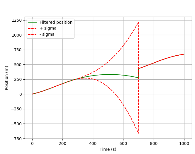
It looks even more interesting if you mask a longer period (300:700).
![filter position without gps signal]()
As you can see the position goes back. It happens because of the transition matrix F, which binds the prediction for position, velocity and acceleration.
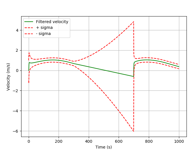
If you have a look at the velocity state, it explains the decreasing position.
![velocity estimation using pykalman and lost gps signal]()
At the time point 300 s the acceleration freezes. The velocity goes down with a constant slope and crosses the 0 value. After this time point the position has to go back.
To plot the velocity use the following code:
velocity_sigma = np.sqrt(filtered_state_covariances[:, 1, 1]);

# plot of the estimated velocity
plt.plot(Time, filtered_state_means[:, 1], "g-", label="Filtered velocity", markersize=1)
plt.plot(Time, filtered_state_means[:, 1] + velocity_sigma, "r--", label="+ sigma", markersize=1)
plt.plot(Time, filtered_state_means[:, 1] - velocity_sigma, "r--", label="- sigma", markersize=1)
plt.grid()
plt.legend(loc="upper left")
plt.xlabel("Time (s)")
plt.ylabel("Velocity (m/s)")
plt.show()


