Baseline correction for spectroscopic data

Question

I am working with Raman spectra, which often have a baseline superimposed with the actual information I am interested in. I therefore would like to estimate the baseline contribution. For this purpose, I implemented a solution from this question.

I do like the solution described there, and the code given works fine on my data. A typical result for calculated data looks like this with the red and orange line being the baseline estimates: Typical result of baseline estimation with calculated data

The problem is: I often have several thousands of spectra which I collect in a pandas DataFrame, each row representing one spectrum. My current solution is to use a for loop to iterate through the data one spectrum at a time. However, this makes the procedure quite slow. As I am rather new to python and just got used to almost not having to use for loops at all thanks to numpy/pandas/scipy, I am looking for a solution which makes it possible to omit this for loop, too. However, the used sparse matrix functions seem to be limited to two dimensions, but I might need three, and I was not able to think of another solution, yet. Does anybody have an idea?

The current code looks like this:

import numpy as np
import pandas as pd
from scipy.signal import gaussian
import matplotlib.pyplot as plt
from scipy import sparse
from scipy.sparse.linalg import spsolve

def baseline_correction(raman_spectra,lam,p,niter=10):
    #according to "Asymmetric Least Squares Smoothing" by P. Eilers and H. Boelens
    number_of_spectra = raman_spectra.index.size
    baseline_data = pd.DataFrame(np.zeros((len(raman_spectra.index),len(raman_spectra.columns))),columns=raman_spectra.columns)

    for ii in np.arange(number_of_spectra):
        curr_dataset = raman_spectra.iloc[ii,:]

        #this is the code for the fitting procedure        
        L = len(curr_dataset)
        w = np.ones(L)
        D = sparse.diags([1,-2,1],[0,-1,-2], shape=(L,L-2))

        for jj in range(int(niter)):
            W = sparse.spdiags(w,0,L,L)
            Z = W + lam * D.dot(D.transpose())
            z = spsolve(Z,w*curr_dataset.astype(np.float64))
            w = p * (curr_dataset > z) + (1-p) * (curr_dataset < z)
        #end of fitting procedure

        baseline_data.iloc[ii,:] = z
    return baseline_data

#the following four lines calculate two sample spectra
wavenumbers = np.linspace(500,2000,100)
intensities1 = 500*gaussian(100,2) + 0.0002*wavenumbers**2
intensities2 = 100*gaussian(100,5) + 0.0001*wavenumbers**2
raman_spectra = pd.DataFrame((intensities1,intensities2),columns=wavenumbers)
#end of smaple spectra calculataion

baseline_data = baseline_correction(raman_spectra,200,0.01)

#the rest is just for plotting the data
plt.figure(1)
plt.plot(wavenumbers,raman_spectra.iloc[0])
plt.plot(wavenumbers,baseline_data.iloc[0])
plt.plot(wavenumbers,raman_spectra.iloc[1])
plt.plot(wavenumbers,baseline_data.iloc[1])

Jemadar

raman_spectra.apply(lambda x: baseline_correction(x), axis=1) will perform row wise calculations. However, you'll have to update baseline_correction – Jacquline

Trenton_M, your suggestion is helpful because it makes the code shorter. However, execution speed is pretty much the same. On a test sample set of 73 spectra the for loop solution takes about 2.21 s and using the apply approach 2.24 s. So I am still looking for a significantly faster solution which would allow to analyze about 3000 spectra preferably within a few seconds. – Jemadar

Have you tried to use SNIP for background detection? Maybe it is faster. – Lengthy

Answer 1

Based on Christian K.´s suggestion, I had a look at the SNIP algorithm for background estimation, details can be found for example here. This is my python code on it:

import numpy as np
import pandas as pd
from scipy.signal import gaussian
import matplotlib.pyplot as plt

def baseline_correction(raman_spectra,niter):

    assert(isinstance(raman_spectra, pd.DataFrame)), 'Input must be pandas DataFrame'

    spectrum_points = len(raman_spectra.columns)
    raman_spectra_transformed = np.log(np.log(np.sqrt(raman_spectra +1)+1)+1)

    working_spectra = np.zeros(raman_spectra.shape)

    for pp in np.arange(1,niter+1):
        r1 = raman_spectra_transformed.iloc[:,pp:spectrum_points-pp]
        r2 = (np.roll(raman_spectra_transformed,-pp,axis=1)[:,pp:spectrum_points-pp] + np.roll(raman_spectra_transformed,pp,axis=1)[:,pp:spectrum_points-pp])/2
        working_spectra = np.minimum(r1,r2)
        raman_spectra_transformed.iloc[:,pp:spectrum_points-pp] = working_spectra

    baseline = (np.exp(np.exp(raman_spectra_transformed)-1)-1)**2 -1
    return baseline

wavenumbers = np.linspace(500,2000,1000)
intensities1 = gaussian(1000,20) + 0.000002*wavenumbers**2
intensities2 = gaussian(1000,50) + 0.000001*wavenumbers**2
raman_spectra = pd.DataFrame((intensities1,intensities2),columns=np.around(wavenumbers,decimals=1))

iterations = 100
baseline_data = baseline_correction(raman_spectra,iterations)


#the rest is just for plotting the data
plt.figure(1)
plt.plot(wavenumbers,raman_spectra.iloc[0])
plt.plot(wavenumbers,baseline_data.iloc[0])
plt.plot(wavenumbers,raman_spectra.iloc[1])
plt.plot(wavenumbers,baseline_data.iloc[1])

It does work and seems to be similarly reliable like the algorithm based on asymmetric least squares smoothing. It is also faster. With 100 iterations, fitting 73 real, measured spectra takes about 1.5 s with generally good results, in contrast to approx. 2.2 for the asymmetric least squares smoothing, so it is an improvement.

What is even better: The required calculation time for 3267 real spectra is only 11.7 s with the SNIP algorithm, whereas it is 1 min 28 s for the asymmetric least squares smoothing. That is probably a result of not having any for loop iterating through every spectrum at a time with the SNIP algorithm.

A typical result of the SNIP algorithm with calculated examples is shown here.

I´m quite happy with this result, so thank you to all contributors for your support!

Update: Thanks to sascha in this question, I found a way to use the asymmetric least squares smoothing without a for loop for iterating through each spectrum, the function for baseline correction looks like this:

def baseline_correction4(raman_spectra,lam,p,niter=10):
    #according to "Asymmetric Least Squares Smoothing" by P. Eilers and H. Boelens
    number_of_spectra = raman_spectra.index.size

    #this is the code for the fitting procedure        
    L = len(raman_spectra.columns)
    w = np.ones(raman_spectra.shape[0]*raman_spectra.shape[1])

    D = sparse.block_diag(np.tile(sparse.diags([1,-2,1],[0,-1,-2],shape=(L,L-2)),number_of_spectra),format='csr')

    raman_spectra_flattened = raman_spectra.values.ravel()

    for jj in range(int(niter)):
        W = sparse.diags(w,format='csr')
        Z = W + lam * D.dot(D.transpose())
        z = spsolve(Z,w*raman_spectra_flattened,permc_spec='NATURAL')
        w = p * (raman_spectra_flattened > z) + (1-p) * (raman_spectra_flattened < z)
    #end of fitting procedure

    baseline_data = pd.DataFrame(z.reshape(number_of_spectra,-1),index=raman_spectra.index,columns=raman_spectra.columns)
    return baseline_data

This approach is based on combining all sparse matrices into one block diagonal sparse matrix. This way, you have to call spsolve only once, no matter how many spectra you have. This results in baseline correction of 73 real spectra in 593 ms (faster than SNIP) and of 3267 real spectra in 32.8 s (slower than SNIP). I hope this will be useful for someone in the future.

Jemadar

Answer 2

New Function

def baseline_correction_new(data: pd.Series, lam: int=200, p: float=0.01, niter: int=10) -> pd.Series:
    #this is the code for the fitting procedure        
    L = len(data)
    w = np.ones(L)
    D = sparse.diags([1,-2,1], [0,-1,-2], shape=(L,L-2))

    for jj in range(int(niter)):
        W = sparse.spdiags(w, 0, L, L)
        Z = W + lam * D.dot(D.transpose())
        z = spsolve(Z, w*data.astype(np.float64))
        w = p * (data > z) + (1-p) * (data < z)

    return pd.Series(z)

Call the new function

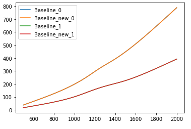
baseline_data_new = raman_spectra.apply(baseline_correction_new, axis=1)

Add column names

baseline_data_new.columns = wavenumbers

Compare

baseline_data.equals(baseline_data_new)
>>> True

Plot

plt.figure(1)
plt.plot(wavenumbers,baseline_data.iloc[0], label='Baseline_0')
plt.plot(wavenumbers,baseline_data_new.iloc[0], label='Baseline_new_0')
plt.plot(wavenumbers,baseline_data.iloc[1], label='Baseline_1')
plt.plot(wavenumbers,baseline_data_new.iloc[1], label='Baseline_new_1')
plt.legend()
plt.show()

Original Method with 3000 rows

%%timeit
baseline_data = baseline_correction(df_int,200,0.01)
>>> 60 s ± 608 ms per loop (mean ± std. dev. of 7 runs, 1 loop each)

apply with 3000 rows

%%timeit
baseline_3000 = df_int.apply(lambda x: baseline_correction_new(x, 200, 0.01), axis=1)
>>> 58.3 s ± 206 ms per loop (mean ± std. dev. of 7 runs, 1 loop each)

• The apply method streamlines the code but only offers a few ms of improvement. Perhaps a route to improvement is to use multiprocessing or 10x Faster Parallel Python Without Python Multiprocessing

Jacquline

Thank you for showing this possibility. This results are similar to what I get. The calculated spectra have about 1000 data points less than measured spectra, thats why speeding the calculation up would be so great. – Jemadar

Unfortunately, I don't have the expertise to improve the correction algorithm. However, if you're on a Mac or Linux pandarallel is a valid option (one of its dependencies isn't currently available for Windows). Perhaps reducing the number of niter. – Jacquline