Python baseline correction library

Question

I am currently working with some Raman Spectra data, and I am trying to correct my data caused by florescence skewing. Take a look at the graph below:

I am pretty close to achieving what I want. As you can see, I am trying to fit a polynomial in all my data whereas I should really just be fitting a polynomial at the local minimas.

Ideally I would want to have a polynomial fitting which when subtracted from my original data would result in something like this:

Are there any built in libs that does this already?

If not, any simple algorithm one can recommend for me?

Rorqual

You could try designing a high path filter by transforming your signal with rfft() and setting the low frequency part to zero. – Fatigued

You should look at the minimum finding techniques in this question: #24656867. Once you have those, you can fit only to the minima to find your baseline correction. – Basque

Answer 1

I found an answer to my question, just sharing for everyone who stumbles upon this.

There is an algorithm called "Asymmetric Least Squares Smoothing" by P. Eilers and H. Boelens in 2005. The paper is free and you can find it on google.

def baseline_als(y, lam, p, niter=10):
  L = len(y)
  D = sparse.csc_matrix(np.diff(np.eye(L), 2))
  w = np.ones(L)
  for i in xrange(niter):
    W = sparse.spdiags(w, 0, L, L)
    Z = W + lam * D.dot(D.transpose())
    z = spsolve(Z, w*y)
    w = p * (y > z) + (1-p) * (y < z)
  return z

Rorqual

works perfectly for me. just quoting from that paper what those parameters are: <<There are two parameters: p for asymmetry and λ for smoothness. Both have to be tuned to the data at hand. We found that generally 0.001 ≤ p ≤ 0.1 is a good choice (for a signal with positive peaks) and 10^2 ≤ λ ≤ 10^9 , but exceptions may occur. In any case one should vary λ on a grid that is approximately linear for log λ>> – Disciplinary

Just a quick question - basically z is the baseline? So the spectrum needs to be subtracted by that array at the end to get baseline corrected? – Nikolas

I cannot find the paper, can you give me the link? Thanks – Mesa

Couldn't find the paper myself, but this article provides a very clear explanation of AsLS and related methods. FWIW, the version they propose worked far better in my case. – Convenience

Answer 2

The following code works on Python 3.6.

This is adapted from the accepted correct answer to avoid the dense matrix diff computation (which can easily cause memory issues) and uses range (not xrange)

import numpy as np
from scipy import sparse
from scipy.sparse.linalg import spsolve

def baseline_als(y, lam, p, niter=10):
  L = len(y)
  D = sparse.diags([1,-2,1],[0,-1,-2], shape=(L,L-2))
  w = np.ones(L)
  for i in range(niter):
    W = sparse.spdiags(w, 0, L, L)
    Z = W + lam * D.dot(D.transpose())
    z = spsolve(Z, w*y)
    w = p * (y > z) + (1-p) * (y < z)
  return z

Rhondarhondda

Answer 3

There is a python library available for baseline correction/removal. It has Modpoly, IModploy and Zhang fit algorithm which can return baseline corrected results when you input the original values as a python list or pandas series and specify the polynomial degree.

Install the library as pip install BaselineRemoval. Below is an example

from BaselineRemoval import BaselineRemoval

input_array=[10,20,1.5,5,2,9,99,25,47]
polynomial_degree=2 #only needed for Modpoly and IModPoly algorithm

baseObj=BaselineRemoval(input_array)
Modpoly_output=baseObj.ModPoly(polynomial_degree)
Imodpoly_output=baseObj.IModPoly(polynomial_degree)
Zhangfit_output=baseObj.ZhangFit()

print('Original input:',input_array)
print('Modpoly base corrected values:',Modpoly_output)
print('IModPoly base corrected values:',Imodpoly_output)
print('ZhangFit base corrected values:',Zhangfit_output)

Original input: [10, 20, 1.5, 5, 2, 9, 99, 25, 47]
Modpoly base corrected values: [-1.98455800e-04  1.61793368e+01  1.08455179e+00  5.21544654e+00
  7.20210508e-02  2.15427531e+00  8.44622093e+01 -4.17691125e-03
  8.75511661e+00]
IModPoly base corrected values: [-0.84912125 15.13786196 -0.11351367  3.89675187 -1.33134142  0.70220645
 82.99739548 -1.44577432  7.37269705]
ZhangFit base corrected values: [ 8.49924691e+00  1.84994576e+01 -3.31739230e-04  3.49854060e+00
  4.97412948e-01  7.49628529e+00  9.74951576e+01  2.34940300e+01
  4.54929023e+01

Surfactant

I tried using the BaselineRemoval library, where the input array is a dataframe column of lists but it was unable to run. Gives the error 'ValueError: setting an array element with a sequence.' – Spall

@Spall Check 1) dimension of array, if it is one dimensional python list object or dataframe['ColumnName'].tolist() it should work. 2) If you are using the latest version of library. If you are still facing issue. create a separate question with example data and post question link here. I will be happy to look into it. – Surfactant

the question is posted here #63634566 – Spall

There is a bug in BaselineRemoval.py, line 27, replace it with: X = np.transpose(np.vstack([input_array_for_poly**k for k in range(degree_for_poly+1)])) – Crenulation

@ffsedd, this bug has now been fixed. – Surfactant

Answer 4

Recently, I needed to use this method. The code from answers works well, but it obviously overuses the memory. So, here is my version with optimized memory usage.

def baseline_als_optimized(y, lam, p, niter=10):
    L = len(y)
    D = sparse.diags([1,-2,1],[0,-1,-2], shape=(L,L-2))
    D = lam * D.dot(D.transpose()) # Precompute this term since it does not depend on `w`
    w = np.ones(L)
    W = sparse.spdiags(w, 0, L, L)
    for i in range(niter):
        W.setdiag(w) # Do not create a new matrix, just update diagonal values
        Z = W + D
        z = spsolve(Z, w*y)
        w = p * (y > z) + (1-p) * (y < z)
    return z

According to my benchmarks bellow, it is also about 1,5 times faster.

%%timeit -n 1000 -r 10 y = randn(1000)
baseline_als(y, 10000, 0.05) # function from @jpantina's answer
# 20.5 ms ± 382 µs per loop (mean ± std. dev. of 10 runs, 1000 loops each)

%%timeit -n 1000 -r 10 y = randn(1000)
baseline_als_optimized(y, 10000, 0.05)
# 13.3 ms ± 874 µs per loop (mean ± std. dev. of 10 runs, 1000 loops each)

NOTE 1: The original article says:

To emphasize the basic simplicity of the algorithm, the number of iterations has been fixed to 10. In practical applications one should check whether the weights show any change; if not, convergence has been attained.

So, it means that the more correct way to stop iteration is to check that ||w_new - w|| < tolerance

NOTE 2: Another useful quote (from @glycoaddict's comment) gives an idea how to choose values of the parameters.

There are two parameters: p for asymmetry and λ for smoothness. Both have to be tuned to the data at hand. We found that generally 0.001 ≤ p ≤ 0.1 is a good choice (for a signal with positive peaks) and 102 ≤ λ ≤ 109, but exceptions may occur. In any case one should vary λ on a grid that is approximately linear for log λ. Often visual inspection is sufficient to get good parameter values.

Newspaperwoman

Would it be correct to use this method for 2D data or are there more suitable implementations? I want to remove baseline from fluorescent microscopy images. It works very well but slow. I am flattening array with ravel and then using your code to find baseline. – Suprematism

Answer 5

I worked the version of the algorithm referenced by glinka in a previous comment, which is an improvement of the penalized weighted linear squares method published in a relatively recent paper. I took Rustam Guliev's code to build this one:

from scipy import sparse
from scipy.sparse import linalg
import numpy as np
from numpy.linalg import norm


def baseline_arPLS(y, ratio=1e-6, lam=100, niter=10, full_output=False):
    L = len(y)

    diag = np.ones(L - 2)
    D = sparse.spdiags([diag, -2*diag, diag], [0, -1, -2], L, L - 2)

    H = lam * D.dot(D.T)  # The transposes are flipped w.r.t the Algorithm on pg. 252

    w = np.ones(L)
    W = sparse.spdiags(w, 0, L, L)

    crit = 1
    count = 0

    while crit > ratio:
        z = linalg.spsolve(W + H, W * y)
        d = y - z
        dn = d[d < 0]

        m = np.mean(dn)
        s = np.std(dn)

        w_new = 1 / (1 + np.exp(2 * (d - (2*s - m))/s))

        crit = norm(w_new - w) / norm(w)

        w = w_new
        W.setdiag(w)  # Do not create a new matrix, just update diagonal values

        count += 1

        if count > niter:
            print('Maximum number of iterations exceeded')
            break

    if full_output:
        info = {'num_iter': count, 'stop_criterion': crit}
        return z, d, info
    else:
        return z

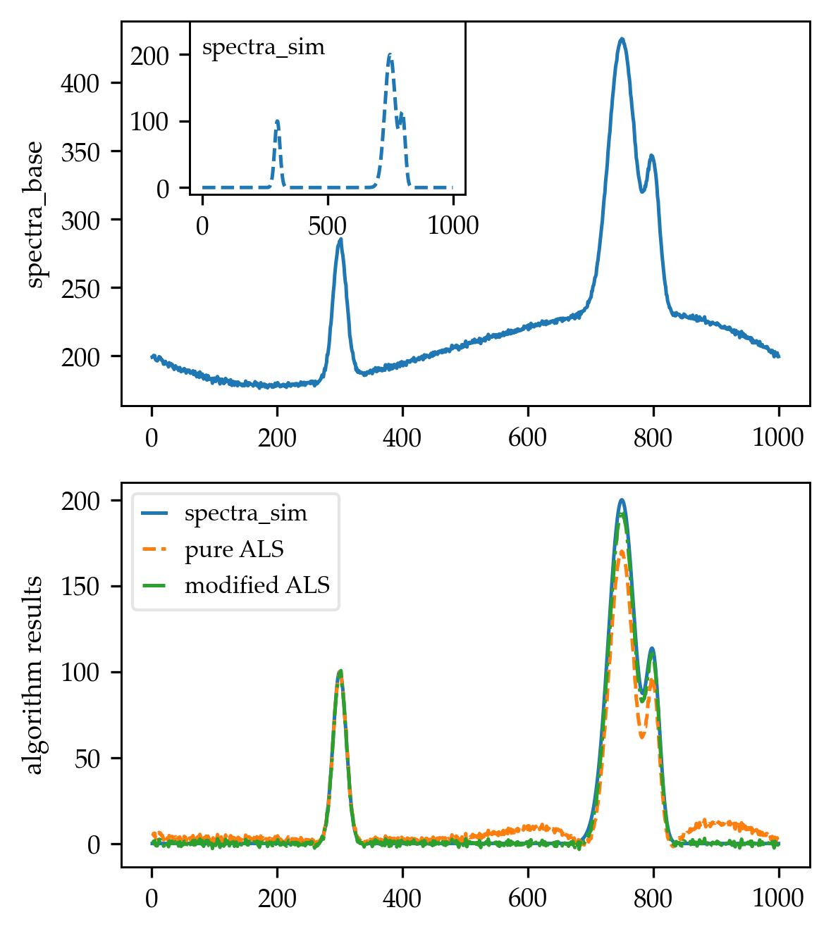
In order to test the algorithm, I created a spectrum similar to the one shown in Fig. 3 of the paper, by first generating a simulated spectra consisting of multiple Gaussian peaks:

def spectra_model(x):
    coeff = np.array([100, 200, 100])
    mean = np.array([300, 750, 800])

    stdv = np.array([15, 30, 15])

    terms = []
    for ind in range(len(coeff)):
        term = coeff[ind] * np.exp(-((x - mean[ind]) / stdv[ind])**2)
        terms.append(term)

    spectra = sum(terms)

    return spectra

x_vals = np.arange(1, 1001)
spectra_sim = spectra_model(x_vals)

Then, I created a third-order interpolating polynomial using 4 points taken directly from the paper:

from scipy.interpolate import CubicSpline
x_poly = np.array([0, 250, 700, 1000])
y_poly = np.array([200, 180, 230, 200])

poly = CubicSpline(x_poly, y_poly)
baseline = poly(x_vals)

noise = np.random.randn(len(x_vals)) * 0.1
spectra_base = spectra_sim + baseline + noise

Finally, I used the baseline correction algorithm to subtract the baseline out of the altered spectra (spectra_base):

 _, spectra_arPLS, info = baseline_arPLS(spectra_base, lam=1e4, niter=10,
                                         full_output=True)

The results were (for reference, I compared with the pure ALS implementation by Rustam Guliev's, using lam = 1e4 and p = 0.001):

Rizzio

thank you daniel. just one question. this can be applied to one single spectrum. if we have 500 spectra (500xrow), how can we do that? – Giesser

Answer 6

I know this is an old question, but I stumpled upon it a few months ago and implemented the equivalent answer using spicy.sparse routines.

# Baseline removal                                                                                            

def baseline_als(y, lam, p, niter=10):                                                                        

    s  = len(y)                                                                                               
    # assemble difference matrix                                                                              
    D0 = sparse.eye( s )                                                                                      
    d1 = [numpy.ones( s-1 ) * -2]                                                                             
    D1 = sparse.diags( d1, [-1] )                                                                             
    d2 = [ numpy.ones( s-2 ) * 1]                                                                             
    D2 = sparse.diags( d2, [-2] )                                                                             

    D  = D0 + D2 + D1                                                                                         
    w  = np.ones( s )                                                                                         
    for i in range( niter ):                                                                                  
        W = sparse.diags( [w], [0] )                                                                          
        Z =  W + lam*D.dot( D.transpose() )                                                                   
        z = spsolve( Z, w*y )                                                                                 
        w = p * (y > z) + (1-p) * (y < z)                                                                     

    return z

Cheers,

Pedro.

Hollo

Answer 7

I've found that the answers provided so far solve the baseline problem, but can be improved further. I will now explain and show how this can be achieved for all implementations that rely on the smoothing spline approach. This approach is taken by most of the answers, including the accepted answer.

General sparse matrices and baselines do not go well together

Basically, all the answers provided so far are correct. However, in terms of runtime, even the optimized algorithms mentioned are not optimal. Most of them solve a sparse matrix for Tikhonov regularization, but the matrix is not just any kind of sparse. Scipy's sparse-module can work with arbitrary sparsity patterns. This makes it a good all-purpose solution, but not the best choice for the systems encountered here.

Systems like the ones solved in the algorithms ((W + lam * D.T @ D) @ baseline = W @ signal) have a special structure. This particular structure is called "banded", i.e., all the nonzero entries are accumulated in a few diagonals around the main diagonal (the "bands"). Here, W is a diagonal weight matrix and D is a banded forward finite difference matrix, so the normal equation system formed for this special case of spline smoothing is banded.

For such systems, a whole bunch of solver algorithms exist, like

• banded Cholesky (fast but numerically instable even though there is regularization; scipy.linalg.solveh_banded)
• banded Partially Pivoted LU-decomposition (more stable, takes ~2x the runtime of banded Cholesky; scipy.linalg.solve_banded)
• the G2B-algorithm which is a special formulation that solves the banded system by a Givens rotation QR-decomposition (most stable, but also the slowest; does not work with the banded normal equation matrix but 2 or more individual banded matrices that are vertically stacked; described in Eldén L., SIAM Journal on Scientific and Statistical Computing, Vol. 5, Iss. 1 (1984), DOI:10.1137/0905017)
• optimised pentadiagonal solvers for the special case when D is a second order finite difference matrix, which can be solved via pentapy (DISCLAIMER: I submitted a Pull request for this package). Unlike all the previously mentioned algorithms, its stability is hard to infer because it solves A @ x = y by factorizing A=LU into a lower triangular matrix L and a unit upper triangular matrix U and solving those by backward/forward substitution. However, instead of L, inv(L) is basically formed directly during the decomposition and inv(L) is dense. During the substitution this does not pose a particular problem because the elements of inv(L) can be represented and applied in a fast recursive fashion. For computing condition numbers however, this might be less ideal because having a dense matrix sort of ruins the idea of using a fast solver that relies on sparsity. Therefore, I'm not 100% sure if there is a simple way to compute the condition number in a similar fashion to LAPACK's ?pbcon (for scipy.linalg.solveh_banded) and ?gbcon (for scipy.linalg.solve_banded), so take that with a grain of salt. However, since it relies on the normal equations method which squares the underlying matrices and thus the condition number, its stability should be around the same order as for Cholesky and Partially Pivoted LU which do the same. QR-decomposition avoids the squaring which makes it far more stable but also slower because the squared matrices here have only roughly 50% of the size of the unsquared problem.

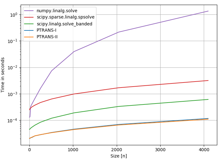
Wow, that's a lot of algorithms. Which of them should one choose? Fortunately, the package pentapy offers an info graphic to compare different solver in terms of speed (the PTRANS solvers are dedicated pentadiagonal solvers):

SciPy's sparse solver is more than 3 times slower than a banded solver and more than 20 times slower than pentapy.
On top of that, the initialisation costs for sparse matrices in SciPy are terribly high. We can time @Rustam Guliev's optimized code for initialisation of the matrix:

import numpy as np
from scipy import sparse

def init_banded_system(y, lam):
    L = len(y)
    D = sparse.diags([1,-2,1],[0,-1,-2], shape=(L,L-2))
    D = lam * D.dot(D.transpose()) # Precompute this term since it does not depend on `w`
    w = np.ones(L)
    W = sparse.spdiags(w, 0, L, L)
    W.setdiag(w) # Do not create a new matrix, just update diagonal values
    Z = W + D

%timeit init_banded_system(np.random.rand(1000), 0.1)
# 1.9 ms ± 448 µs per loop (mean ± std. dev. of 7 runs, 100 loops each)

In 2 ms, scipy.linalg.solve_banded can solve a system of n=1000 roughly 10x and pentapy can even solve it 50x (in theory, not with Python loops though).
Banded matrices however, can be initialised in virtually no time as a dense NumPy-Array by making use of dedicated storage conventions, basically with one diagonal per row ¹⁾.
Since the spline-based baseline corrections require some iterations, having a slow initialisation and solve is usually not acceptable in practice. From my experience with applications in spectroscopy, taking longer than 10 ms on limited hardware can already be too slow when spectra are to be analysed real-time and baseline correction is only a preprocessing step (usually a few thousand data points for a single spectrum).

So all in all, using general sparse matrices is not the state of the art for solving baseline problems via spline smoothing.

¹⁾ Note that this was optimised for LAPACK, i.e., a Fortran program where 2D-Arrays are stored such that the individual columns are coherent (row index changes fastest). However, NumPy uses C order where the individual rows are coherent (column index changes fastest). So when invoking scipy.linalg.solve_banded, which calls LAPACK under the hood, on a C order Array, some memory rearrangement is involved. For pentapy - being written in Cython - this does not happen, but it still relies on a format similar to the LAPACK convention. Therefore, the initial access to the memory is not fully optimal. This fact makes the banded solvers in Python slower than they have to be. For writing customised routines for banded matrices, this should be considered. For C order, a cache-friendly implementation will require to store the individual diagonals as columns of an Array and not as rows.

Python packages

You don't need to reinvent the wheel here. The package pybaselines provides a function-based interface for 1D- and 2D-baseline correction with a very good documentation and a wide variety of algorithms. It relies on scipy.linalg.solve_banded under the hood. On top of that, it offers a runtime integration for pentapy and will make use of its fast solvers when they are installed and applicable for the problem to solve.
In case, you want to build a data processing pipeline within the scikit-learn framework commonly used for data analytics, the package chemotools also offers baseline correction algorithms, even though not as many as pybaselines. As of June 2024, it is still using scipy.sparse, but a pull request to switch for banded solvers and pentapy is in review (DISCLAIMER: I'm a collaborator for this project and submitted the PR).

Since there are many algorithms implemented in these packages, I can only forward to their respective documentations. However, for the automated choice of the smoothing parameter lam, pybaselines' erPLS is a very good bet and my secret favourite for all those who read this for (or only this part).

Edit June 12, 2024
I clarified a mistake in how pentapy works. In contrast to what I wrote initially, it does indeed perform a factorization. However, the fact that the condition number is not straightforward to infer remains unchanged.

Paronomasia

Thanks a lot for your review. I will check out these packages. – Curtiscurtiss

You are welcome! Please let me know if I can clarify anything in a better way! Also, please note that I edited a mistake I made in the description of how pentapy works. I just realised it today. In case, you are interested in the linear algebra details about it, you might find this issue and this issue interesting. – Paronomasia

In fact, I'm rather on the application side. As a physicist I encounter different types of spectra (Raman, Fluorescene, both mixed, XPS, Mass specs, FTIR, Atomic emission, ...) and I was wondering if you were aware of a table or an overview article suggesting a type of baseline for these different spectra types? – Curtiscurtiss

I'm working a lot with FTIR-spectroscopy and in this context I read a lot about other spectroscopic techniques and how they tackle the problem. From my experience, the baseline will always have noise and this renders a lot of algorithms useless, most prominently ASLS, because their estimates will often lie below the true baseline because the noise spikes below it. If you look through the pybaselines-docs, there are plots of examples and the first one has a noisy baseline. I would only pick those algorithms where the baseline in that plot coincides with the true baseline. – Paronomasia

One good example is ARPLS which works quite nicely for noise. Once you picked one algorithm that suites you well (I would not make it a philosophic question, many good algorithms give more or less the same result), I highly recommend to apply them within the optimization framework. Then, you facilitate the choice of hyperparamters which is in my experience the biggest source of errors. – Paronomasia

One word auf caution: all the baseline algorithms are data-driven and thus need to "see" the baseline somewhere in the signal. If your true baseline is not showing anywhere or rarely, e.g., because there are peaks that are not baseline-resolved located everywhere on top of it, the algorithms will all produce garbage baselines. Tackling such cases requires parametric approaches where you have to model the true baseline based on knowledge about your system. – Paronomasia

Thanks for your comments MothNik, at the moment I work with FTIR spectra too. As my spectrometer is not N2-purged I have a problem with the air lines. The 'atmospheric correction' feature of my spectrometer is not always satisfying so sometimes I prefer just cutting out the air bands... But then I have data with interrupted support and the baseline algorithms I tested do not perform well on this. Any ideas how to treat spectra with a big gap? – Curtiscurtiss

You probably mean the water vapour lines? They are problematic. There is a patent by Perkin Elmer where they use HITRAN for simulating the water vapour lines for multiple conditions (humity, pressure, temperature). Then, they simulate the instrument function's effect on it, i.e., the broadening by the finite resolution (cutting out frequencies of the Fourier transform) and beam divergence (convolution with a moving average after the x-axis was log-transformed). Finally, they perform a least squares fit. That's still a state of the art approach, but I think the patent can be circumvented. – Paronomasia

Sorry, I didn't understand the comment fully. You see and cut out the water vapour peaks in the absorbance (A) or the energy/intensity spectrum (I or I_0)? I think I need further information on this and see the original data to fully grasp the problem and how you attempt the solution. Unfortunately, the comment section is a bit too small for the topic of atmospheric correction which is still prominent in research today. Especially open source solutions are scarce. – Paronomasia

Here is the patent. For simulating spectra of gases in high fidelity in Python, one can use radis. – Paronomasia

Usually my data is saved as (wavenumber (cm-1), transmission(%)). Even after the atmospheric correction the data from 1990-1340 cm-1 is noisier than I would like. So I can cut it out of the numpy array, give the cut wavenumber-axis to the Baseline object and try some baselines (arpls), however the data close to the cut is not at the same level and does not have the same slope (maybe due to differences in the substrates). Thus the baselines do not stick well to the data close to the cut even if there is no absorption peak there. – Curtiscurtiss

Did not have the time to try it yet, but maybe filling the cut with some smooth differentiable function and then giving the hole thing to the Baseline object may help. But maybe there is an easier and quicker method? – Curtiscurtiss

You can also try giving the wavenumbers where you performed the cut out weights of zero. For ARPLS or other spline-based approaches, this will have the effect that these values are interpolated based on the complete dataset, which usually works reasonably well. If I remember correctly, pybaselines supports this, but I'm not sure 🤔 – Paronomasia