Way to contour outer edge of selected grid region in Python
Asked Answered
C

2

6

I have the following code:

import numpy as np
import matplotlib.pyplot as plt

x = np.linspace(-np.pi/2, np.pi/2, 30)
y = np.linspace(-np.pi/2, np.pi/2, 30)
x,y = np.meshgrid(x,y)

z = np.sin(x**2+y**2)[:-1,:-1]

fig,ax = plt.subplots()
ax.pcolormesh(x,y,z)

Which gives this image: enter image description here

Now lets say I want to highlight the edge certain grid boxes:

highlight = (z > 0.9)

I could use the contour function, but this would result in a "smoothed" contour. I just want to highlight the edge of a region, following the edge of the grid boxes.

The closest I've come is adding something like this:

highlight = np.ma.masked_less(highlight, 1)

ax.pcolormesh(x, y, highlight, facecolor = 'None', edgecolors = 'w')

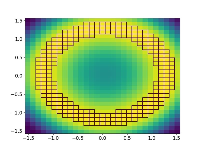
Which gives this plot: enter image description here

Which is close, but what I really want is for only the outer and inner edges of that "donut" to be highlighted.

So essentially I am looking for some hybrid of the contour and pcolormesh functions - something that follows the contour of some value, but follows grid bins in "steps" rather than connecting point-to-point. Does that make sense?

Side note: In the pcolormesh arguments, I have edgecolors = 'w', but the edges still come out to be blue. Whats going on there?

EDIT: JohanC's initial answer using add_iso_line() works for the question as posed. However, the actual data I'm using is a very irregular x,y grid, which cannot be converted to 1D (as is required for add_iso_line().

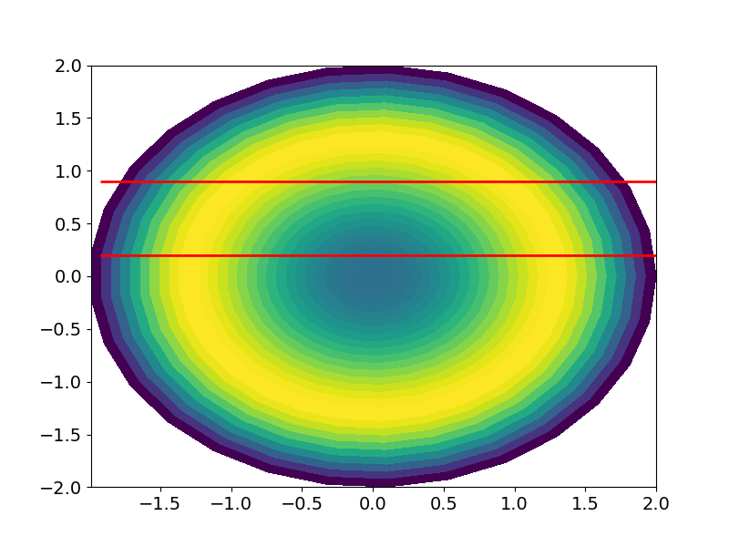
I am using data which has been converted from polar coordinates (rho, phi) to cartesian (x,y). The 2D solution posed by JohanC does not appear to work for the following case:

import numpy as np
import matplotlib.pyplot as plt
from scipy import ndimage

def pol2cart(rho, phi):
    x = rho * np.cos(phi)
    y = rho * np.sin(phi)
    return(x, y)

phi = np.linspace(0,2*np.pi,30)
rho = np.linspace(0,2,30)

pp, rr = np.meshgrid(phi,rho)

xx,yy = pol2cart(rr, pp)

z = np.sin(xx**2 + yy**2)

scale = 5
zz = ndimage.zoom(z, scale, order=0)

fig,ax = plt.subplots()
ax.pcolormesh(xx,yy,z[:-1, :-1])

xlim = ax.get_xlim()
ylim = ax.get_ylim()
xmin, xmax = xx.min(), xx.max()
ymin, ymax = yy.min(), yy.max()
ax.contour(np.linspace(xmin,xmax, zz.shape[1]) + (xmax-xmin)/z.shape[1]/2,
           np.linspace(ymin,ymax, zz.shape[0]) + (ymax-ymin)/z.shape[0]/2,
           np.where(zz < 0.9, 0, 1), levels=[0.5], colors='red')
ax.set_xlim(*xlim)
ax.set_ylim(*ylim)

enter image description here

Comprise answered 17/8, 2020 at 21:25 Comment(2)
Yes, it is clear and very useful questionMicrometeorite
z[z>0.9] = 0 or z[z>0.9] = 1 to change the values so they are different. Note that pyplot automatically is asigning a color map. You may want to use a grayscale color map. Or you may want to just use cv2.imshow() to see it in grayscale. Then you can convert to 3 channels and make the emphasis red z1=cv2.merge([z,z,z]) and then z1[z>0.9]=(255,255,255)Hypallage
P
1

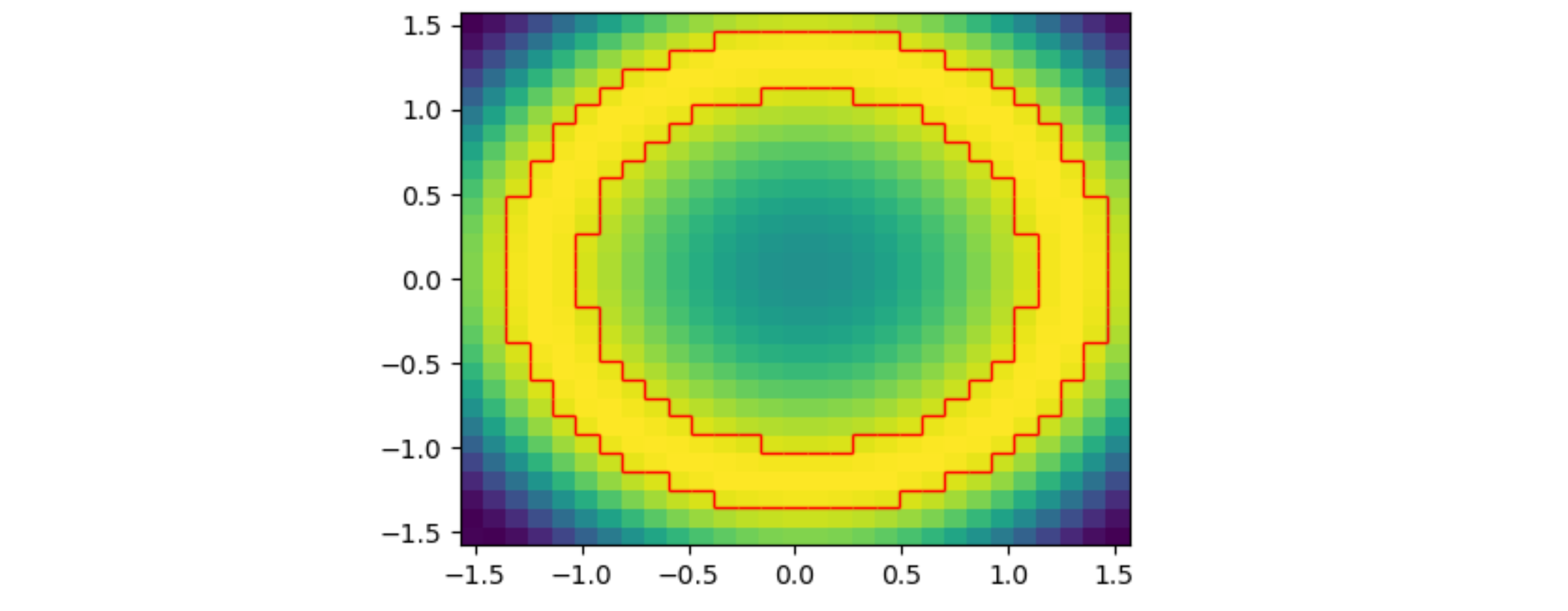
This post shows a way to draw such lines. As it is not straightforward to adapt to the current pcolormesh, the following code demonstrates a possible adaption. Note that the 2d versions of x and y have been renamed, as the 1d versions are needed for the line segments.

import numpy as np
import matplotlib.pyplot as plt
from matplotlib.collections import LineCollection

x = np.linspace(-np.pi / 2, np.pi / 2, 30)
y = np.linspace(-np.pi / 2, np.pi / 2, 30)
xx, yy = np.meshgrid(x, y)

z = np.sin(xx ** 2 + yy ** 2)[:-1, :-1]

fig, ax = plt.subplots()
ax.pcolormesh(x, y, z)

def add_iso_line(ax, value, color):
    v = np.diff(z > value, axis=1)
    h = np.diff(z > value, axis=0)

    l = np.argwhere(v.T)
    vlines = np.array(list(zip(np.stack((x[l[:, 0] + 1], y[l[:, 1]])).T,
                               np.stack((x[l[:, 0] + 1], y[l[:, 1] + 1])).T)))
    l = np.argwhere(h.T)
    hlines = np.array(list(zip(np.stack((x[l[:, 0]], y[l[:, 1] + 1])).T,
                               np.stack((x[l[:, 0] + 1], y[l[:, 1] + 1])).T)))
    lines = np.vstack((vlines, hlines))
    ax.add_collection(LineCollection(lines, lw=1, colors=color))

add_iso_line(ax, 0.9, 'r')
plt.show()

resulting plot

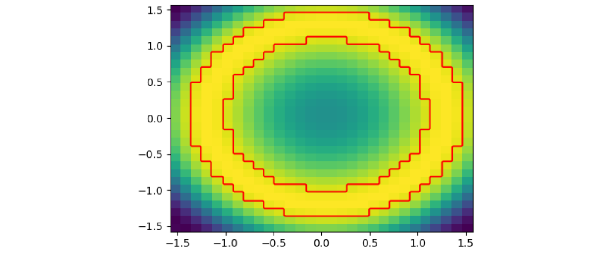
Here is an adaption of the second answer, which can work with only 2d arrays:

import numpy as np
import matplotlib.pyplot as plt
from matplotlib.collections import LineCollection
from scipy import ndimage

x = np.linspace(-np.pi / 2, np.pi / 2, 30)
y = np.linspace(-np.pi / 2, np.pi / 2, 30)
x, y = np.meshgrid(x, y)

z = np.sin(x ** 2 + y ** 2)

scale = 5
zz = ndimage.zoom(z, scale, order=0)

fig, ax = plt.subplots()
ax.pcolormesh(x, y,  z[:-1, :-1] )
xlim = ax.get_xlim()
ylim = ax.get_ylim()
xmin, xmax = x.min(), x.max()
ymin, ymax = y.min(), y.max()
ax.contour(np.linspace(xmin,xmax, zz.shape[1]) + (xmax-xmin)/z.shape[1]/2,
           np.linspace(ymin,ymax, zz.shape[0]) + (ymax-ymin)/z.shape[0]/2,
           np.where(zz < 0.9, 0, 1), levels=[0.5], colors='red')
ax.set_xlim(*xlim)
ax.set_ylim(*ylim)
plt.show()

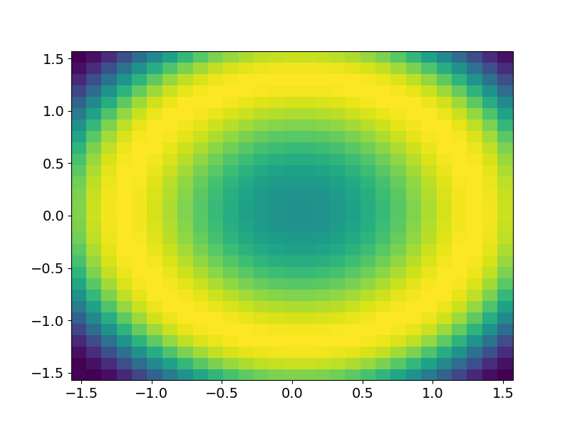
second example

Pivotal answered 17/8, 2020 at 22:18 Comment(3)
Ok, so this answers the question as posed. However, I guess I simplified it too much. In the dataset I'm actually working with, x and y are not a on a regular grid - I can't change them into 1-D. Should I make a new question?Comprise
You probably can extract the 1d versions from the 2d versions. Something like x1d = x[0,:] and y1d = y[:,0]. Feel free to extend your current question (or add a new one).Pivotal
The proposed 2D solution does not work for my case. I've updated the original question with anew example.Comprise
M
0

I'll try to refactor add_iso_line method in order to make it more clear an open for optimisations. So, at first, there comes a must-do part:

import numpy as np
import matplotlib.pyplot as plt
from matplotlib.collections import LineCollection

x = np.linspace(-np.pi/2, np.pi/2, 30)
y = np.linspace(-np.pi/2, np.pi/2, 30)
x, y = np.meshgrid(x,y)
z = np.sin(x**2+y**2)[:-1,:-1]

fig, ax = plt.subplots()
ax.pcolormesh(x,y,z)
xlim, ylim = ax.get_xlim(), ax.get_ylim()
highlight = (z > 0.9)

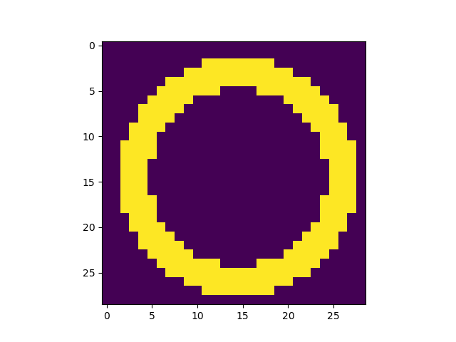
Now highlight is a binary array that looks like this: enter image description here After that we can extract indexes of True cells, look for False neighbourhoods and identify positions of 'red' lines. I'm not comfortable enough with doing it in a vectorised manner (like here in add_iso_line method) so just using simple loop:

lines = []
cells = zip(*np.where(highlight))
for x, y in cells:
    if x == 0 or highlight[x - 1, y] == 0: lines.append(([x, y], [x, y + 1]))
    if x == highlight.shape[0] or highlight[x + 1, y] == 0: lines.append(([x + 1, y], [x + 1, y + 1]))
    if y == 0 or highlight[x, y - 1] == 0: lines.append(([x, y], [x + 1, y]))
    if y == highlight.shape[1] or highlight[x, y + 1] == 0: lines.append(([x, y + 1], [x + 1, y + 1]))

And, finally, I resize and center coordinates of lines in order to fit with pcolormesh:

lines = (np.array(lines) / highlight.shape - [0.5, 0.5]) * [xlim[1] - xlim[0], ylim[1] - ylim[0]]
ax.add_collection(LineCollection(lines, colors='r'))
plt.show()

In conclusion, this is very similar to JohanC solution and, in general, slower. Fortunately, we can reduce amount of cells significantly, extracting contours only using python-opencv package:

import cv2
highlight = highlight.astype(np.uint8)
contours, hierarchy = cv2.findContours(highlight, cv2.RETR_TREE, cv2.CHAIN_APPROX_NONE)
cells = np.vstack(contours).squeeze()

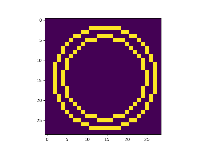
This is an illustration of cells being checked: enter image description here

Micrometeorite answered 18/8, 2020 at 3:48 Comment(0)

© 2022 - 2024 — McMap. All rights reserved.