Particle Dynamics
Asked Answered
I

3

6

I am modelling a particle in 3D space.

Particle Interpolation

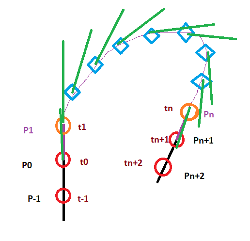
{0} The particle starts at time t0 from a known position P0 with a velocity V0. The velocity is computed using its known previous position of P-1 at t-1.

{1} The particle is targeted to go to P1 at t1 with a known velocity of V1.

{..} The particle moves as fast as it can, without jerks (C1 continuous) bound by a set of constraints that clamp the acceleration along x, y and z independently. The maximum acceleration/deceleration along x, y and z are known and are Xa, Ya, and Za. The max rate of change of acceleration along x, y and z are defined by Xr, Yr, and Zr.

{n} After an unknown number of time steps it reaches Pn at some time (say tn) with a velocity of Vn.

{n+1} It moves to Pn+1 at tn+1.

The problem I have is to compute the minimum time for the transition from P0 to Pn and to generate the intermediate positions and velocity directions thereof. A secondary goal is to accelerate smoothly instead of applying acceleration that results in jerks.

Current Approach:

  1. find the dimension {x, y or z} that will take the longest to align from start P0 to end Pn. This will be the critical dimension and will determine the total time. This is fairly straightforward and I can write something to this effect.

  2. interpolate smoothly without jitters from P0 to Pn in all dimensions such that the velocity at Pn is as expected. I am not sure, how to approach this.

Any inputs/physics engines that already do this will be useful. It is a commercial project and I cannot put dependencies on large 3rd party libraries with restrictive licenses.

Note: Particle at P0 and Pn have little or no acceleration.

Isolationism answered 22/2, 2018 at 16:6 Comment(18)
Have you looked into calculus of variations? It can be used to solve similar problemsSarah
So if the initial state is known, and velocities / accelerations are computed from the previous state, wouldn't the path be 100% deterministic? If so, how do you define a "minimum" time? Also, if the number of time steps is unknown, how would you know Pn?Fransen
Is it V0 = P0 - P-1 or V0 = P1 - P0? Does the velocity at some point lead you to the next point, or from the previous one to the current one?Quinlan
@Fransen The acceleration isn't determined from previous states.Quinlan
But if you compute the velocity based on the position history only, that's equivalent to computing the acceleration.Fransen
The intermediate positions are clearly unknown here. As I understand it, the problem is to find the acceleration at each point that would lead to the shortest path from (P0, V0) to (Pn, Vn).Quinlan
@meow, I know the start states and the end states and nothing in between. The idea is to minimise the time of the steps in betweenIsolationism
@Nelfeal, to keep the terminology simple, at P0, velocity is V0. The instantaneous velocity at P0 is computed by its past and not its future.Isolationism
@user308..., I know nothing about calculus of variations. Do you have a link? Looked at Wiki and it sure is deep.Isolationism
@Ram, I learned the basics in a dynamics course. Unfortunately I don't have a link since the course was mostly done on the blackboard. Wikipedia gives a decent overview, but nothing about how to do itSarah
Searching for "Lagrange multipliers with inequality constraints" might give some insight into thisFransen
This is very complex. Lets look at 1 dimension. If you have p0 at 0 and pn at 1, both with velocity 10, 0 acceleration and max acceleration change of 1, then you will overshoot pn, and you have to come to a stop, go to the left, stop again at a point where you have enough space to get to a velocity of 10 again with 0 acceleration.Jibe
Yes it is inherently complex. There are classes of curves that can do this. It is how to apply then to this problem which is the key.Isolationism
What I think is a little strange is that you have a max change of acceleration and a max acceleration, so if you are at max acceleration then you have to get higher velocity until acceleration comes down to 0. Wouldn't it be easier to have a max velocity change and a max velocity only? This should also give smooth curves.Jibe
Max acceleration is absolute value and also holds limits for max deceleration. If the particle is at max velocity, it cant drop to zero velocity as this is limited by max acceleration.Isolationism
@Isolationism but there is no max velocity, only a max acceleration in the problem description. This means that there is no bound on the max velocity. So are those actually max velocity and max velocity change and not acceleration?Jibe
So you know P0 and V0 and you want to get to Pfinal and Vfinal in the minimum amount of time?Landmeier
I am still looking to improve and complete my second answer. Do you have any updates on your side? Have you implemented something?Quinlan
Q
3

After playing around with some ideas, I came up with another solution, more accurate and probably faster, if done correctly, than that of my previous answer. It is however quite complicated and requires quite a bit of maths, although not very complex maths. Moreover, this is a work in progress: I am still investigating some areas. Nonetheless, from what I've tried, it does already produce very good results.

The problem

Definitions and goal

Throughout this answer, p[n] refers to the position of the nth point, v[n] to its velocity, a[n] to its acceleration, and j[n] to its jerk (the derivative of acceleration). The velocity of the nth point depends only on its position and that of the previous point. Similarly for acceleration and jerk, but with the points velocity and acceleration, respectively.

We have a start point and an end point, respectively p[0] and p[n], both with associated velocities v[0] and v[n]. The goal is to place n-1 points in between, with an arbitrary n, such that, along the X, Y, and Z axes, the absolute values of acceleration and jerk at any of these points (and at p[n]) are below some limits, respectively aMaxX, aMaxY, and aMaxZ for acceleration, and jMaxX, jMaxY, and jMaxZ for jerk.

What we want to find is the values of p[i] for all i ∈ [1; n-1]. Because p[i] = p[i-1] + v[i], this is the same as finding v[i]. By the same reasoning, with v[i] = v[i-1] + a[i] and a[i] = a[i-1] + j[i], it is also the same as finding a[i] or j[i].

a[0] and a[n+1] are assumed to be zero.

Observations and simplifications

Because the problem's constraints are independant of the dimension, we can solve for each of the three dimensions separately, as long as the number of points obtained in each case is the same. Therefore, I am only going to solve the one-dimensional version of the problem, using aMax and jMax, irrespective of the axis.

*[WIP]* Determine the worst case to solve first, then solve the other ones, knowing the number of points.

The actual positions of the two given points are irrelevant, what matters is the relative distance between them, which we can define as P = p[n] - p[0]. Let's also define the ranges R = [1; n] and R* = [1; n+1].

Because of the discrete nature of the problem, we can obtain the following equations. Note that ∑{i∈R}(x[i]) is the sum of all x[i] for i∈R.

Ⓐ ∑{i∈R}(v[i]) = P
Ⓑ ∑{i∈R}(a[i]) = v[n] - v[0]
Ⓧ ∑{i∈R*}(j[i]) = 0

Ⓧ comes from the assumption that a[0] = a[n+1] = 0.
From Ⓐ and v[i] = v[i-1] + a[i], i∈R, we can deduce:

Ⓒ ∑{i∈R}((n+1-i)*a[i]) = P - n*v[0]

By the same logic, from Ⓑ, Ⓒ, and a[i] = a[i-1] + j[i], i∈R, we can deduce:

Ⓨ ∑{i∈R}((n+1-i)*j[i]) = v[n] - v[0]
Ⓩ ∑{i∈R}(T[n+1-i]*j[i]) = P - n*v[0]

Here, T[n] is the nth triangular number, defined by T[n] = n*(n+1)/2.

The equations Ⓧ, Ⓨ, and Ⓩ are the relevant ones for the next parts.

The approach

In order to minimize n, we can start with a small value of n (1, 2?) and find a solution. Then, if max{i∈R}(abs(a[i])) > aMax or max{i∈R}(abs(j[i])) > jMax, we can increment n and repeat the process.

*[WIP]* Find a lower bound for n to avoid unnecessary calculations from small values of n. Or estimate the correct value of n and pinpoint it by testing solutions.

Finding a solution requires finding the values of j[i] for all i∈R*. I have yet to find an optimal form for j[i], but defining j*[i], r[i] and s[i] such that
j[i] = j*[i] + r[i]v[0] + s[i]v[n]
works quite well.

*[WIP]* Find a better form for j[i]

By doing that, we transform our n-1 unknowns (j[i], i∈R, note that j[n+1] = -∑{i∈R}(j[i])) into 3(n-1) easier to find unknowns. Here are a few things we can deduce right now from Ⓧ, Ⓨ, and Ⓩ.

∑{i∈R*}(r[i]) = 0
∑{i∈R*}(s[i]) = 0
∑{i∈R}((n+1-i)*r[i]) = -1
∑{i∈R}((n+1-i)*s[i]) = 1
∑{i∈R}(T(n+1-i)*r[i]) = -n
∑{i∈R}(T(n+1-i)*s[i]) = 0

As a reminder, here are Ⓧ, Ⓨ, and Ⓩ.

Ⓧ ∑{i∈R*}(j[i]) + j[n+1] = 0
Ⓨ ∑{i∈R}((n+1-i)*j[i]) = v[n] - v[0]
Ⓩ ∑{i∈R}(T[n+1-i]*j[i]) = P - n*v[0]

The goal now is to find adequate special cases to help us determine these unknowns.

The special cases

v[0] = v[n] = 0

By playing with values of jerk, I observed that taking all of j[i], i∈R* as part of a parabola yields excellent results for minimizing both jerk and acceleration. Although it isn't the best possible fit, I haven't found better yet.

The intuition behind values of jerk coming from a parabola is that, if the values of position are to follow a polynomial, then its degree must be at least 5, and can be 5. This is easier to understand if you think about the values of velocity following a 4th degree polynomial. The constraints that v[0] and v[n] are set, a[0] = a[n+1] = 0, and that its integral over [0; n] must equal P, this polynomial must have a degree of at least 4. This holds for both continuous and dicrete cases. Finally, it seems that taking the smallest degree leads to a smoother jerk as well as making it easier to calculate.

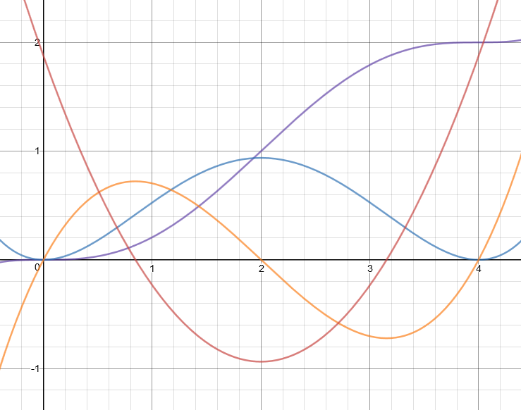
Here is an example of a continuous case where the position is in purple, the velocity in blue, the acceleration in yellow and the jerk in red.

Example curves for position, velocity, acceleration, and jerk

In case you want to play with this, here is how to define the position curve in terms of n, p[0], p[n], v[0], and v[n] (the other ones are simply derivatives).

a = (-3(v[n]+v[0]) + 6(p[n]-p[0])) / n^5
b = (n(7v[n]+8v[0]) - 15(p[n]-p[0])) / n^4
c = (-n(4v[n]+6v[0]) + 10(p[n]-p[0])) / n^3
p[x] = ax^5 + bx^4 + cx^3 + v[0]x + p[0]

If v[0] = v[n] = 0, then j[i] = j*[i], i∈R*. That means that the values j*[i] follow a quadratic polynomial. So we want to find α, β, and γ such that Ⓟ holds.

Ⓟ j*[i] = αi^2 + βi + γ, i∈R*

From Ⓧ, Ⓨ, and Ⓩ follow these equations.

α*∑{i∈R*}(i^2) + β*∑{i∈R*}(i) + c*∑{i∈R*}(1) = 0
α*∑{i∈R}((n+1-i)*i^2) + β*∑{i∈R}((n+1-i)*i) + c*∑{i∈R}(n+1-i) = 0
α*∑{i∈R}(T(n+1-i)*i^2) + β*∑{i∈R}(T(n+1-i)*i) + c*∑{i∈R}(T(n+1-i)) = P

Solving this system gives α, β, and γ, which can be used with Ⓟ to calculate j*[i], i∈R*. Note that j*[i] = j*[n+2-i], so only the upper half of the calculations need to be done.

v[0] = v[n] = 1/n

If v[0] = v[n] = 1/n, then j[i] = 0, i∈R*. This means that Ⓠ holds.

Ⓠ r[i] + s[i] = -n*j[i], i∈R*

v[0] = 0, j[i∈L] = J, j[h] = 0, j[i∈U] = -J

L and U are respectively the lower and upper halves of R*, and h is the value in between, if n+1 is odd. In other words:

if n is odd:
L = [1; (n+1)/2]
U = [(n+3)/2; n+1]
if n is even:
L = [1; n/2]
h = n/2+1
U = [n/2+2; n]

This special case corresponds to the maximum overall acceleration between p[0] and p[n] while minimizing abs(j[i]), i∈R*. Here, Ⓩ gives us the following equation.

∑{i∈R}(T[n+1-i]*j[i]) = P
∑{i∈L}(T[n+1-i])*j[1] + ∑{i∈U}(T[n+1-i])*j[n+1] = P
j[1] = P / [ ∑{i∈L}(T[n+1-i]) - ∑{i∈U}(T[n+1-i]) ]

This gives j[1], and so every j[i], i∈R*. We can then calculate v[n] using Ⓨ.

Putting the pieces together

Each special case gives us, for some values of v[0], v[n] and P, a relation of the form
αj*[i] + βr[i] + γs[i] = δ.
By treating three special cases (assuming they are not similar, meaning the do not give the same relation), we have a system of three equations that, once solved, gives the values of j*[i], r[i] and s[i] for all i∈R*.

As a result, we can calculate, for each value of n, values of j[i] depending on v[0], v[n] and P. They can be precalculated, which means testing them for any value of n can be very fast. Thereby, we can very quicklyt find a good estimate for the fewest amount of points needed in the trajectory, as well as a good approximation of the best trajectory possible, as long as we have precalculated values up to a sufficiently large value of n.

Quinlan answered 3/3, 2018 at 14:9 Comment(0)
Q
5

If I understand correctly, you have a point (P0, V0), with V0 = P0 - P-1, and a point (Pn, Vn), with Vn = Pn - Pn-1, and you want to find the fewest intermediate points by adjusting the acceleration at each time step.

Let's define the acceleration at ti: Ai = Vi - Vi-1, with abs(Ai) <= mA. Here, since the problem is axis-independant, abs is the member-wise absolute instead of the norm (or vector magnitude), and mA is the maximum acceleration vector, positive in each dimension. Let's also consider that Pn > P0 (member-wise).

From that, we get Vi = Vi-1 + Ai and so Pi = Pi-1 + Vi-1 + Ai.

If you need to go from some point to another in the fastest way possible, the obvious thing to do, whatever the initial velocity, is accelerate as much as possible until you reach the goal. However, since your problem is discrete and you have a terminal velocity Vn, using that method will probably lead too far and with a different terminal velocity.

However, you can do the same thing in reverse, starting from the end point. And if you start simultaneously from both points, you will make two paths crossing each other in each dimension (not necessarily crossing in 3D, but, in each dimension, the relative direction of both paths changes at some "crossing" point).

Let's take a one-dimensional example. (P0, V0) = (0, -2) and (Pn, Vn) = (35, -1), and mA = 1.
The first path, with Ai = mA, goes like this:

(0, -2) -> (-1, -1) -> (-1, 0) -> (0, 1) -> (2, 2) ->
(5, 3) -> (9, 4) -> (14, 5) -> (20, 6) -> (27, 7) -> ...

The second path, with Ai = -mA but in reverse, goes like this:

(35, -1) <- (36, 0) <- (36, 1) <- (35, 2) <- (33, 3) <-
(30, 4) <- (26, 5) <- (21, 6) <- (15, 7) <- ...

You can see the paths cross with the same velocity somewhere between 20 and 21. That gives you the fastest acceleration and deceleration parts of the path you need, but the two parts aren't connected. However, it's easy to connect them by finding the closest points of same velocity; let's call these points Pq and Pr. Here, Pq = (20, 6) and Pr = (21, 6). Since that velocity is calculated between current and previous points, take the point before Pq (Pq-1, or (14, 5) in the example) and the point Pr, and try connecting them.

If Pq >= Pr >= Pq - 2mA, then you can connect them directly by taking Pq-1 unchanged, and Pr with Vr = Pr - Pq-1.

Else, take Pq-2 and Pr-1 (where Vr-1 = Vr - mA, because it's in reverse) and try connecting those by adding intermediate points. Since these points have a velocity difference of mA, you can search only for intermediate points with the same velocity Vs such that Vq-2 <= Vs <= Vr-1.

If you still can't find a solution, then take Pq-3 and Pr-2 and repeat the process with more intermediate points.

In the example I took, Pq < Pr, so we have to try with Pq-2 = (9, 4) and Pr-1 = (26, 5). We can connect those with a sequence of 3 points, for example (9, 4) -> (13, 4) -> (17, 4) -> (21, 4) -> (26, 5).

In any case, this method will give you the smallest amount of intermediate points, meaning the fastest path between P0 and Pn.

If you then want to reduce jerk, then you can forget the points calculated previously and do an interpolation with the number of points you now know to be minimal.

Quinlan answered 22/2, 2018 at 17:57 Comment(8)
This answer reminds me of two of the answers used for this: #40623815Sarah
@Nelfel, in your approach each dim produces a solution with a different num of steps or n. I am not clear how this converges to a single set of points and velocities.Isolationism
True. However, you can easily add more points in a particular dimension by scaling down the velocities at each point. Or just use the method to get the number of points and do an interpolation.Quinlan
tried this. Did not give the results as expected. This approach accelerates and decelerates all dimensions at highest allowed rate even when it is not required. Further, at the terminal point the velocity comes along with maximum acceleration and to bring that acceleration from max to 0 is no feasible.Isolationism
Then you need to define your problem more clearly. You haven't mentioned that last requirement.Quinlan
The velocity at Pn and beyond is fixed. If the transition brings an acceleration component at Pn that will not lead to Pn+1 then it is not meeting the end conditions.Isolationism
This is not a problem unless you want acceleration to be somewhat continuous. If Vn is close to the wanted Vn+1, then having An+1 close to zero meets the end conditions in term of position and velocity. If you cannot go from An = -mA to An+1 ≈ 0, then a constraint is missing from your problem description. Is there a limit on the jerk value? That would correspond to a "continuous" acceleration for discrete points.Quinlan
Your answer produces a very jerky interim set of points and is far from what I want. Since I understood what I want from implementing this approach, I m up voting your answer. But it still is not the desired approach. I have updated the question with my understanding.Isolationism
Q
3

After playing around with some ideas, I came up with another solution, more accurate and probably faster, if done correctly, than that of my previous answer. It is however quite complicated and requires quite a bit of maths, although not very complex maths. Moreover, this is a work in progress: I am still investigating some areas. Nonetheless, from what I've tried, it does already produce very good results.

The problem

Definitions and goal

Throughout this answer, p[n] refers to the position of the nth point, v[n] to its velocity, a[n] to its acceleration, and j[n] to its jerk (the derivative of acceleration). The velocity of the nth point depends only on its position and that of the previous point. Similarly for acceleration and jerk, but with the points velocity and acceleration, respectively.

We have a start point and an end point, respectively p[0] and p[n], both with associated velocities v[0] and v[n]. The goal is to place n-1 points in between, with an arbitrary n, such that, along the X, Y, and Z axes, the absolute values of acceleration and jerk at any of these points (and at p[n]) are below some limits, respectively aMaxX, aMaxY, and aMaxZ for acceleration, and jMaxX, jMaxY, and jMaxZ for jerk.

What we want to find is the values of p[i] for all i ∈ [1; n-1]. Because p[i] = p[i-1] + v[i], this is the same as finding v[i]. By the same reasoning, with v[i] = v[i-1] + a[i] and a[i] = a[i-1] + j[i], it is also the same as finding a[i] or j[i].

a[0] and a[n+1] are assumed to be zero.

Observations and simplifications

Because the problem's constraints are independant of the dimension, we can solve for each of the three dimensions separately, as long as the number of points obtained in each case is the same. Therefore, I am only going to solve the one-dimensional version of the problem, using aMax and jMax, irrespective of the axis.

*[WIP]* Determine the worst case to solve first, then solve the other ones, knowing the number of points.

The actual positions of the two given points are irrelevant, what matters is the relative distance between them, which we can define as P = p[n] - p[0]. Let's also define the ranges R = [1; n] and R* = [1; n+1].

Because of the discrete nature of the problem, we can obtain the following equations. Note that ∑{i∈R}(x[i]) is the sum of all x[i] for i∈R.

Ⓐ ∑{i∈R}(v[i]) = P
Ⓑ ∑{i∈R}(a[i]) = v[n] - v[0]
Ⓧ ∑{i∈R*}(j[i]) = 0

Ⓧ comes from the assumption that a[0] = a[n+1] = 0.
From Ⓐ and v[i] = v[i-1] + a[i], i∈R, we can deduce:

Ⓒ ∑{i∈R}((n+1-i)*a[i]) = P - n*v[0]

By the same logic, from Ⓑ, Ⓒ, and a[i] = a[i-1] + j[i], i∈R, we can deduce:

Ⓨ ∑{i∈R}((n+1-i)*j[i]) = v[n] - v[0]
Ⓩ ∑{i∈R}(T[n+1-i]*j[i]) = P - n*v[0]

Here, T[n] is the nth triangular number, defined by T[n] = n*(n+1)/2.

The equations Ⓧ, Ⓨ, and Ⓩ are the relevant ones for the next parts.

The approach

In order to minimize n, we can start with a small value of n (1, 2?) and find a solution. Then, if max{i∈R}(abs(a[i])) > aMax or max{i∈R}(abs(j[i])) > jMax, we can increment n and repeat the process.

*[WIP]* Find a lower bound for n to avoid unnecessary calculations from small values of n. Or estimate the correct value of n and pinpoint it by testing solutions.

Finding a solution requires finding the values of j[i] for all i∈R*. I have yet to find an optimal form for j[i], but defining j*[i], r[i] and s[i] such that
j[i] = j*[i] + r[i]v[0] + s[i]v[n]
works quite well.

*[WIP]* Find a better form for j[i]

By doing that, we transform our n-1 unknowns (j[i], i∈R, note that j[n+1] = -∑{i∈R}(j[i])) into 3(n-1) easier to find unknowns. Here are a few things we can deduce right now from Ⓧ, Ⓨ, and Ⓩ.

∑{i∈R*}(r[i]) = 0
∑{i∈R*}(s[i]) = 0
∑{i∈R}((n+1-i)*r[i]) = -1
∑{i∈R}((n+1-i)*s[i]) = 1
∑{i∈R}(T(n+1-i)*r[i]) = -n
∑{i∈R}(T(n+1-i)*s[i]) = 0

As a reminder, here are Ⓧ, Ⓨ, and Ⓩ.

Ⓧ ∑{i∈R*}(j[i]) + j[n+1] = 0
Ⓨ ∑{i∈R}((n+1-i)*j[i]) = v[n] - v[0]
Ⓩ ∑{i∈R}(T[n+1-i]*j[i]) = P - n*v[0]

The goal now is to find adequate special cases to help us determine these unknowns.

The special cases

v[0] = v[n] = 0

By playing with values of jerk, I observed that taking all of j[i], i∈R* as part of a parabola yields excellent results for minimizing both jerk and acceleration. Although it isn't the best possible fit, I haven't found better yet.

The intuition behind values of jerk coming from a parabola is that, if the values of position are to follow a polynomial, then its degree must be at least 5, and can be 5. This is easier to understand if you think about the values of velocity following a 4th degree polynomial. The constraints that v[0] and v[n] are set, a[0] = a[n+1] = 0, and that its integral over [0; n] must equal P, this polynomial must have a degree of at least 4. This holds for both continuous and dicrete cases. Finally, it seems that taking the smallest degree leads to a smoother jerk as well as making it easier to calculate.

Here is an example of a continuous case where the position is in purple, the velocity in blue, the acceleration in yellow and the jerk in red.

Example curves for position, velocity, acceleration, and jerk

In case you want to play with this, here is how to define the position curve in terms of n, p[0], p[n], v[0], and v[n] (the other ones are simply derivatives).

a = (-3(v[n]+v[0]) + 6(p[n]-p[0])) / n^5
b = (n(7v[n]+8v[0]) - 15(p[n]-p[0])) / n^4
c = (-n(4v[n]+6v[0]) + 10(p[n]-p[0])) / n^3
p[x] = ax^5 + bx^4 + cx^3 + v[0]x + p[0]

If v[0] = v[n] = 0, then j[i] = j*[i], i∈R*. That means that the values j*[i] follow a quadratic polynomial. So we want to find α, β, and γ such that Ⓟ holds.

Ⓟ j*[i] = αi^2 + βi + γ, i∈R*

From Ⓧ, Ⓨ, and Ⓩ follow these equations.

α*∑{i∈R*}(i^2) + β*∑{i∈R*}(i) + c*∑{i∈R*}(1) = 0
α*∑{i∈R}((n+1-i)*i^2) + β*∑{i∈R}((n+1-i)*i) + c*∑{i∈R}(n+1-i) = 0
α*∑{i∈R}(T(n+1-i)*i^2) + β*∑{i∈R}(T(n+1-i)*i) + c*∑{i∈R}(T(n+1-i)) = P

Solving this system gives α, β, and γ, which can be used with Ⓟ to calculate j*[i], i∈R*. Note that j*[i] = j*[n+2-i], so only the upper half of the calculations need to be done.

v[0] = v[n] = 1/n

If v[0] = v[n] = 1/n, then j[i] = 0, i∈R*. This means that Ⓠ holds.

Ⓠ r[i] + s[i] = -n*j[i], i∈R*

v[0] = 0, j[i∈L] = J, j[h] = 0, j[i∈U] = -J

L and U are respectively the lower and upper halves of R*, and h is the value in between, if n+1 is odd. In other words:

if n is odd:
L = [1; (n+1)/2]
U = [(n+3)/2; n+1]
if n is even:
L = [1; n/2]
h = n/2+1
U = [n/2+2; n]

This special case corresponds to the maximum overall acceleration between p[0] and p[n] while minimizing abs(j[i]), i∈R*. Here, Ⓩ gives us the following equation.

∑{i∈R}(T[n+1-i]*j[i]) = P
∑{i∈L}(T[n+1-i])*j[1] + ∑{i∈U}(T[n+1-i])*j[n+1] = P
j[1] = P / [ ∑{i∈L}(T[n+1-i]) - ∑{i∈U}(T[n+1-i]) ]

This gives j[1], and so every j[i], i∈R*. We can then calculate v[n] using Ⓨ.

Putting the pieces together

Each special case gives us, for some values of v[0], v[n] and P, a relation of the form
αj*[i] + βr[i] + γs[i] = δ.
By treating three special cases (assuming they are not similar, meaning the do not give the same relation), we have a system of three equations that, once solved, gives the values of j*[i], r[i] and s[i] for all i∈R*.

As a result, we can calculate, for each value of n, values of j[i] depending on v[0], v[n] and P. They can be precalculated, which means testing them for any value of n can be very fast. Thereby, we can very quicklyt find a good estimate for the fewest amount of points needed in the trajectory, as well as a good approximation of the best trajectory possible, as long as we have precalculated values up to a sufficiently large value of n.
Quinlan answered 3/3, 2018 at 14:9 Comment(0)
P
1

Answer

I suggest you to take following function :

X(n) = Xstart + Vxstart n+ (-6xstart+3Vxstart+6xend-3Vxend+c/2) n^2 + (8xstart+3Vxstart-8xend+5Vxend-c) n^3 + (-3Xstart-Vxstart+3xend-2Vxend+c/2) n^4

(for each coordinate X,Y,Z)

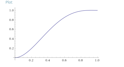
Here are some graphs of what this gives, I took c=3 for each samples:

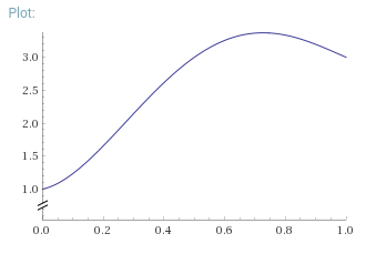
For xstart=1, vstart=1, xend=3, vstart=-2, this gives :

X(n)= 1 + n + 16 n^2 -25 n^3 + 10 n^4

enter image description here

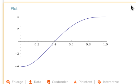
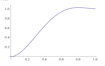
For xstart = -4, vstart =-4, xend = 4, vend = 0, this gives :

(-4 -4n +61n^2 -78n^3 + 29yn^4)

enter image description here

where c is a number from 0.1 to 5, it is up to you to decide, the higher c will be, the faster the function will go to that point (but it might have to turn back if c > 4). (See graphs below).

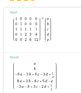
The polynomial comes from following calculation : where a=x0,b=v0,c=xe,d=v2,e=the magic constant

enter image description here

Explanation

Based on Nelfeal's answer, my idea was to try to solve the given problem with polynomials.

We can change the problem as to define a new Axis which goes in the P[last]-P[0], to have the problem reduced to dimension 1.

We can think about the problem in continuous mathematics instead of discrete mathematics (eg use functions instead of sequences), and go back to the discrete world which is just a special case of the continuous.

We can change the unit for time and space so that the time is 1 and the distance is 1, so that the problem is simplified to

Find a function 𝒇 which satisfies the following :

  1. 𝒇(0) = 0 and 𝒇(1) = 1
  2. 𝒇'(0) = 0 and 𝒇'(1) = 0
  3. For x∈ℝ |𝒇''(x)| < c, where c is the max speed

We have

P(X) = ∑{i∈ℕ} Ai Xi

P'(X) = ∑{i∈ℕ} (i+1) Ai+1 Xi

P''(X) = ∑{i∈ℕ} (i+2)(i+1) Ai+2 Xi

We need :

  1. P(0) = 0
  2. P(1) = 1
  3. P'(0) = 0
  4. P'(1) = 0
  5. -c <= P''(x) <= c

Thus it means :

a0 = 0 (from 1.) a1 = 0 (from 3.)

P(1) = ∑{i∈ℕ} Ai = 1

P'(1) = ∑{i∈ℕ} (i+1) Ai = 0

P''(x) = ∑{i∈ℕ} (i+2)(i+1) Ai Xi in [-c,c]

The third equation is the most complex one, and can be simplified by saying that P(1) = c.

We will have c vary to see what changes.

After inverting a 3x3 matrix, we get following result :

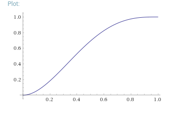
P(x) = (c/2+6) x^2 - (c+8) x^3 + (c/2+3) x^4

For c=0.15, this gives :

enter image description here

For c=1, this gives:

enter image description here

For c=4, we see a bounce back :

enter image description here

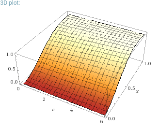
If we take c from 0.1 to 6, we get following 3d graph :

enter image description here

Note that we have solved this for polynomals of degree 4, but you might do the same things to higher degrees (up to 10 if you want to) to get more possibilities in your functions.

Phonics answered 3/3, 2018 at 17:22 Comment(0)

© 2022 - 2024 — McMap. All rights reserved.