Piecewise regression with a straight line and a horizontal line joining at a break point
Asked Answered
A

2

5

I want to do a piecewise linear regression with one break point, where the 2nd half of the regression line has slope = 0. There are examples of how to do a piecewise linear regression, such as here. The problem I'm having is I'm not clear how to fix the slope of half of the model to be 0.

I tried

lhs <- function(x) ifelse(x < k, k-x, 0)
rhs <- function(x) ifelse(x < k, 0, x-k)
fit <- lm(y ~ lhs(x) + rhs(x)) 

where k is the break point, but the segment on the right is not a flat / horizontal one.

I want to constrain the slope of the second segment at 0. I tried:

fit <- lm(y ~ x * (x < k) + x * (x > k))

but again, I'm not sure how to get the second half to have a zero slope.

Any help is greatly appreciated.


My own solution

I have a solution thanks to the comment below. Here's the code that I use to optimize and then plot the fit:

x <- c(1, 2, 3, 1, 2, 1, 6, 1, 2, 3, 2, 1, 4, 3, 1)
y <- c(0.041754212, 0.083491254, 0.193129615, 0.104249201, 0.17280516, 
0.154342335, 0.303370501, 0.025503008, 0.123934121, 0.191486527, 
0.183958737, 0.156707866, 0.31019215, 0.281890206, 0.25414608)

range_x <- max(x) - min(x)
intervals <- 1000
coef1 <- c()
coef2 <- c()
r2 <- c()

for (i in 1:intervals) {
  k <- min(x) + (i-1) * (range_x / intervals)     
  x2 = (x - k) * (x < k)
  fit <- lm(y ~ x2)
  coef1[i] <- summary(fit)$coef[1]
  coef2[i] <- summary(fit)$coef[2]
  r2[i] <- summary(fit)$r.squared
  }

best_r2 <- max(r2)   # get best r squared
pos <- which.max(r2)                                          
best_k <- min(x) + (pos - 1) * (range_x / intervals)

plot(x, y) 
curve(coef1[pos] - best_k * coef2[pos] + coef2[pos] * x,
      from=min(x), to=best_k, add = TRUE)
segments(best_k, coef1[pos], max(x), coef1[pos])

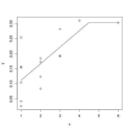
my solution

Accusatorial answered 5/5, 2015 at 18:11 Comment(2)
What do your data look like?Mopey
@Mopey x = c(1, 2, 3, 1, 2, 1, 6, 1, 2, 3, 2, 1, 4, 3, 1) y = c(0.041754212, 0.083491254, 0.193129615, 0.104249201, 0.17280516, 0.154342335, 0.303370501, 0.025503008, 0.123934121, 0.191486527, 0.183958737, 0.156707866, 0.31019215, 0.281890206, 0.025414608) I realize these data aren't great for the fit i'm describing but that's kind of the point...Accusatorial
E
5

There is a very similar thread on Stack Overflow: Piecewise regression with a quadratic polynomial and a straight line joining smoothly at a break point. The only difference is that we now consider:

parametrization

It turns out that functions est, choose.c and pred defined in my answer need not be changed at all; we only need to modify getX to return the design matrix for your piecewise regression:

getX <- function (x, c) cbind("beta0" = 1, "beta1" = pmin(x - c, 0))

Now, we follow the code in toy example to fit a model to your data:

x <- c(1, 2, 3, 1, 2, 1, 6, 1, 2, 3, 2, 1, 4, 3, 1)
y <- c(0.041754212, 0.083491254, 0.193129615, 0.104249201, 0.17280516, 
0.154342335, 0.303370501, 0.025503008, 0.123934121, 0.191486527, 
0.183958737, 0.156707866, 0.31019215, 0.281890206, 0.25414608)

x ranges from 1 to 6, so we consider

c.grid <- seq(1.1, 5.9, 0.05)
fit <- choose.c(x, y, c.grid)
fit$c
# 4.5

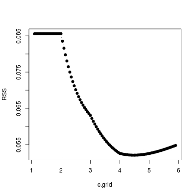
choose c by minimizing RSS

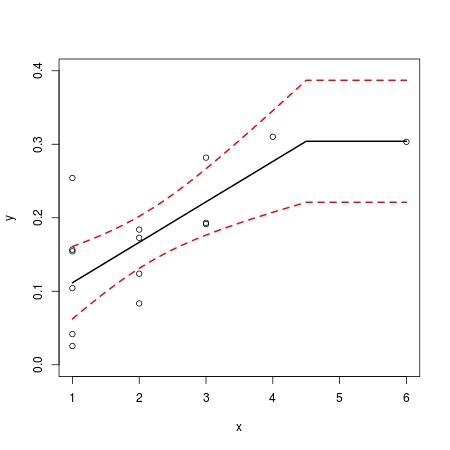
Finally we make prediction plot:

x.new <- seq(1, 6, by = 0.1)
p <- pred(fit, x.new)
plot(x, y, ylim = c(0, 0.4))
matlines(x.new, p[,-2], col = c(1,2,2), lty = c(1,2,2), lwd = 2)

prediction plot

We have rich information in the fitted model:

str(fit)
#List of 12
# $ coefficients : num [1:2] 0.304 0.055
# $ residuals    : num [1:15] -0.06981 -0.08307 -0.02844 -0.00731 0.00624 ...
# $ fitted.values: num [1:15] 0.112 0.167 0.222 0.112 0.167 ...
# $ R            : num [1:2, 1:2] -3.873 0.258 9.295 -4.37
# $ sig2         : num 0.00401
# $ coef.table   : num [1:2, 1:4] 0.3041 0.055 0.0384 0.0145 7.917 ...
#  ..- attr(*, "dimnames")=List of 2
#  .. ..$ : chr [1:2] "beta0" "beta1"
#  .. ..$ : chr [1:4] "Estimate" "Std. Error" "t value" "Pr(>|t|)"
# $ aic          : num -34.2
# $ bic          : num -39.5
# $ c            : num 4.5
# $ RSS          : num 0.0521
# $ r.squared    : num 0.526
# $ adj.r.squared: num 0.49

For example, we can inspect coefficients summary table:

fit$coef.table
#        Estimate Std. Error  t value     Pr(>|t|)
#beta0 0.30406634 0.03840657 7.917039 2.506043e-06
#beta1 0.05500095 0.01448188 3.797915 2.216095e-03
Exponible answered 27/11, 2016 at 3:28 Comment(0)
V
2

Try making the variables outside the expression.

x2 = (x-k)*(x>k)
lm( y ~ x2)

Alternatively, you can use I()

lm(y~ I((x-k)*(x>k)))

I() takes whatever is inside literally and ignores other possible (mis)interpretations with whatever function it is inside of.

If you don't have a well-defined k, then you will have to optimize something like deviance over different values of k.

Viand answered 5/5, 2015 at 18:16 Comment(2)
I'm confused about how this sets the slope of half of the line to 0?Accusatorial
One half of the line will always be 0, because when(x<=k), (x>k) is FALSE, and FALSE * anynumber is 0. When x==k, it will be still zero because the function should be continuous. After that, (x-k) will increase at a constant rate.Viand

© 2022 - 2024 — McMap. All rights reserved.