Piecewise regression with a quadratic polynomial and a straight line joining smoothly at a break point
Asked Answered
S

3

5

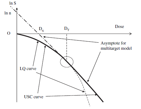
I want to fit a piecewise linear regression with one break point xt, such that for x < xt we have a quadratic polynomial and for x >= xt we have a straight line. Two pieces should join smoothly, with continuity up to 1st derivative at xt. Here's picture of what it may look like:

piecewise regression

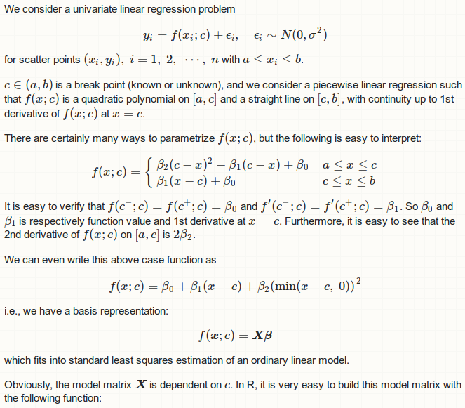
I have parametrize my piecewise regression function as:

regression function

where a, b, c and xt are parameters to be estimated.

I want to compare this model with a quadratic polynomial regression over the whole range in terms of adjusted R-squared.

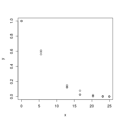
Here is my data:

y <- c(1, 0.59, 0.15, 0.078, 0.02, 0.0047, 0.0019, 1, 0.56, 0.13, 
0.025, 0.0051, 0.0016, 0.00091, 1, 0.61, 0.12, 0.026, 0.0067, 
0.00085, 4e-04)

x <- c(0, 5.53, 12.92, 16.61, 20.3, 23.07, 24.92, 0, 5.53, 12.92, 
16.61, 20.3, 23.07, 24.92, 0, 5.53, 12.92, 16.61, 20.3, 23.07, 
24.92)

scatter plot

My attempt goes as follows, for a known xt:

z <- pmax(0, x - xt)
x1 <- pmin(x, xt)
fit <- lm(y ~  x1 + I(x1 ^ 2) + z - 1)

But the straight line does not appear to be tangent to the quadratic polynomial at xt. Where am I doing wrong?


Similar questions:

Strickland answered 9/9, 2016 at 19:47 Comment(3)
And the question is? If you are not sure how to go about this, maybe this would be of use: R for Ecologists: Putting Together a Piecewise Regression.Unlettered
This is a question for Cross Validated, as it refers to a Statistical model and not programming. That being said, you're going to want to use a dummy variable to nest the two models in one equation. For example. y = I + ax + bx^2*(I-1), were I takes a value of 1 when x>=xt and 0 otherwisePromotion
Are you after continuity and continuity of the first derivative? Is finding the breakpoint your main problem or is defining the predictors your main problem?Sennacherib
G
6

In this section I will be demonstrating a reproducible example. Please make sure you have sourced functions defined in the other answer.

## we first generate a true model
set.seed(0)
x <- runif(100)  ## sample points on [0, 1]
beta <- c(0.1, -0.2, 2)  ## true coefficients
X <- getX(x, 0.6)  ## model matrix with true break point at 0.6
y <- X %*% beta + rnorm(100, 0, 0.08)  ## observations with Gaussian noise
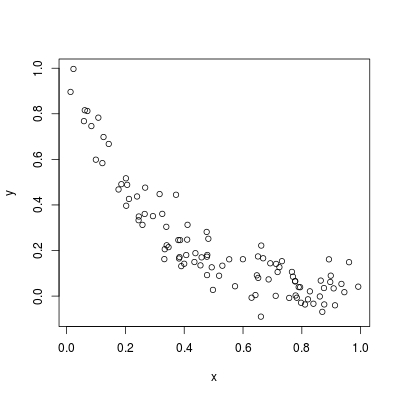
plot(x, y)

scatter plot

Now, assume we don't know c, and we would like to search on a evenly spaced grid:

c.grid <- seq(0.1, 0.9, 0.05)
fit <- choose.c(x, y, c.grid)
fit$c

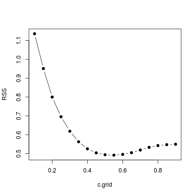
choose c

RSS has chosen 0.55. This is slightly different from the true value 0.6, but from the plot we see that RSS curve does not vary much between [0.5, 0.6] so I am happy with this.

The resulting model fit contains rich information:

#List of 12
# $ coefficients : num [1:3] 0.114 -0.246 2.366
# $ residuals    : num [1:100] 0.03279 -0.01515 0.21188 -0.06542 0.00763 ...
# $ fitted.values: num [1:100] 0.0292 0.3757 0.2329 0.1087 0.0263 ...
# $ R            : num [1:3, 1:3] -10 0.1 0.1 0.292 2.688 ...
# $ sig2         : num 0.00507
# $ coef.table   : num [1:3, 1:4] 0.1143 -0.2456 2.3661 0.0096 0.0454 ...
#  ..- attr(*, "dimnames")=List of 2
#  .. ..$ : chr [1:3] "beta0" "beta1" "beta2"
#  .. ..$ : chr [1:4] "Estimate" "Std. Error" "t value" "Pr(>|t|)"
# $ aic          : num -240
# $ bic          : num -243
# $ c            : num 0.55
# $ RSS          : num 0.492
# $ r.squared    : num 0.913
# $ adj.r.squared: num 0.911

We can extract the summary table for coefficients:

fit$coef.table
#        Estimate  Std. Error   t value     Pr(>|t|)
#beta0  0.1143132 0.009602697 11.904286 1.120059e-20
#beta1 -0.2455986 0.045409356 -5.408546 4.568506e-07
#beta2  2.3661097 0.169308226 13.975161 5.730682e-25

Finally, we want to see some prediction plot.

x.new <- seq(0, 1, 0.05)
p <- pred(fit, x.new)

head(p)
#           fit     se.fit       lwr       upr
#[1,] 0.9651406 0.02903484 0.9075145 1.0227668
#[2,] 0.8286400 0.02263111 0.7837235 0.8735564
#[3,] 0.7039698 0.01739193 0.6694516 0.7384880
#[4,] 0.5911302 0.01350837 0.5643199 0.6179406
#[5,] 0.4901212 0.01117924 0.4679335 0.5123089
#[6,] 0.4009427 0.01034868 0.3804034 0.4214819

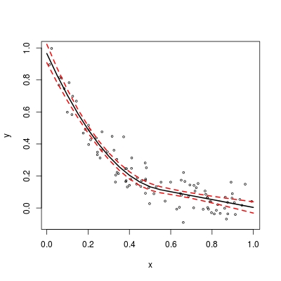
We can make a plot:

plot(x, y, cex = 0.5)
matlines(x.new, p[,-2], col = c(1,2,2), lty = c(1,2,2), lwd = 2)

confidence band

Greed answered 26/11, 2016 at 10:44 Comment(0)
G
6

This is an excellent exercise (maybe hard) to digest the theory and implementation of linear models. My answer will contain two parts:

  • Part 1 (this one) introduces the parametrization I use and how this piecewise regression reduces to an ordinary least square problem. R functions including model estimation, break point selection and prediction are provided.
  • Part 2 (the other one) demonstrates a toy, reproducible example on how to use those functions I have defined.

I have to use a different parametrization because the one you gave in your question is wrong! Your parametrization only ensures continuity of function value, but not the first derivative! That is why your fitted line is not tangent to the fitted quadratic polynomial at xt.


Parametrization

## generate design matrix
getX <- function (x, c) {
  x <- x - c
  cbind("beta0" = 1, "beta1" = x, "beta2" = pmin(x, 0) ^ 2)
  }

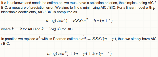
Using AIC to select c

Using RSS to select c

grid search to find c

Function est below wraps up .lm.fit (for maximum efficiency) for estimation and inference of a model, at a given c:

## `x`, `y` give data points; `c` is known break point
est <- function (x, y, c) {
  ## model matrix
  X <- getX(x, c)
  p <- dim(X)[2L]
  ## solve least squares with QR factorization
  fit <- .lm.fit(X, y)
  ## compute Pearson estimate of `sigma ^ 2`
  r <- c(fit$residuals)
  n <- length(r)
  RSS <- c(crossprod(r))
  sig2 <- RSS / (n - p)
  ## coefficients summary table
  beta <- fit$coefficients
  R <- "dimnames<-"(fit$qr[1:p, ], NULL)
  Rinv <- backsolve(R, diag(p))
  se <- sqrt(rowSums(Rinv ^ 2) * sig2)
  tstat <- beta / se
  pval <- 2 * pt(abs(tstat), n - p, lower.tail = FALSE)
  tab <- matrix(c(beta, se, tstat, pval), nrow = p, ncol = 4L,
                dimnames = list(dimnames(X)[[2L]], 
                c("Estimate", "Std. Error", "t value", "Pr(>|t|)")))
  ## 2 * negative log-likelihood
  nega2logLik <- n * log(2 * pi * sig2) + (n - p)
  ## AIC / BIC
  aic <- nega2logLik + 2 * (p + 1)
  bic <- nega2logLik + log(n) * (p + 1)
  ## multiple R-squared and adjusted R-squared
  TSS <- c(crossprod(y - sum(y) / n))
  r.squared <- 1 - RSS / TSS
  adj.r.squared <- 1 - sig2 * (n - 1) / TSS
  ## return
  list(coefficients = beta, residuals = r, fitted.values = c(X %*% beta),
       R = R, sig2 = sig2, coef.table = tab, aic = aic, bic = bic, c = c,
       RSS = RSS, r.squared = r.squared, adj.r.squared = adj.r.squared)
  }

As you can see, it also returns various summary as if summary.lm has been called. Now let's write another wrapper function choose.c. It sketch RSS against c.grid and return the best model with selected c.

choose.c <- function (x, y, c.grid) {
  if (is.unsorted(c.grid)) stop("'c.grid' in not increasing")
  ## model list
  lst <- lapply(c.grid, est, x = x, y = y)
  ## RSS trace
  RSS <- sapply(lst, "[[", "RSS")
  ## verbose
  plot(c.grid, RSS, type = "b", pch = 19)
  ## find `c` / the model minimizing `RSS`
  lst[[which.min(RSS)]]
  }

So far so good. To complete the story, we also want a predict routine.

pred <- function (model, x.new) {
  ## prediction matrix
  X <- getX(x.new, model$c)
  p <- dim(X)[2L]
  ## predicted mean
  fit <- X %*% model$coefficients
  ## prediction standard error
  Qt <- forwardsolve(t(model$R), t(X))
  se <- sqrt(colSums(Qt ^ 2) * model$sig2)
  ## 95%-confidence interval
  alpha <- qt(0.025, length(model$residuals) - p)
  lwr <- fit + alpha * se
  upr <- fit - alpha * se
  ## return
  matrix(c(fit, se, lwr, upr), ncol = 4L,
         dimnames = list(NULL, c("fit", "se", "lwr", "upr")))
  }
Greed answered 26/11, 2016 at 10:40 Comment(0)
G
6

In this section I will be demonstrating a reproducible example. Please make sure you have sourced functions defined in the other answer.

## we first generate a true model
set.seed(0)
x <- runif(100)  ## sample points on [0, 1]
beta <- c(0.1, -0.2, 2)  ## true coefficients
X <- getX(x, 0.6)  ## model matrix with true break point at 0.6
y <- X %*% beta + rnorm(100, 0, 0.08)  ## observations with Gaussian noise
plot(x, y)

scatter plot

Now, assume we don't know c, and we would like to search on a evenly spaced grid:

c.grid <- seq(0.1, 0.9, 0.05)
fit <- choose.c(x, y, c.grid)
fit$c

choose c

RSS has chosen 0.55. This is slightly different from the true value 0.6, but from the plot we see that RSS curve does not vary much between [0.5, 0.6] so I am happy with this.

The resulting model fit contains rich information:

#List of 12
# $ coefficients : num [1:3] 0.114 -0.246 2.366
# $ residuals    : num [1:100] 0.03279 -0.01515 0.21188 -0.06542 0.00763 ...
# $ fitted.values: num [1:100] 0.0292 0.3757 0.2329 0.1087 0.0263 ...
# $ R            : num [1:3, 1:3] -10 0.1 0.1 0.292 2.688 ...
# $ sig2         : num 0.00507
# $ coef.table   : num [1:3, 1:4] 0.1143 -0.2456 2.3661 0.0096 0.0454 ...
#  ..- attr(*, "dimnames")=List of 2
#  .. ..$ : chr [1:3] "beta0" "beta1" "beta2"
#  .. ..$ : chr [1:4] "Estimate" "Std. Error" "t value" "Pr(>|t|)"
# $ aic          : num -240
# $ bic          : num -243
# $ c            : num 0.55
# $ RSS          : num 0.492
# $ r.squared    : num 0.913
# $ adj.r.squared: num 0.911

We can extract the summary table for coefficients:

fit$coef.table
#        Estimate  Std. Error   t value     Pr(>|t|)
#beta0  0.1143132 0.009602697 11.904286 1.120059e-20
#beta1 -0.2455986 0.045409356 -5.408546 4.568506e-07
#beta2  2.3661097 0.169308226 13.975161 5.730682e-25

Finally, we want to see some prediction plot.

x.new <- seq(0, 1, 0.05)
p <- pred(fit, x.new)

head(p)
#           fit     se.fit       lwr       upr
#[1,] 0.9651406 0.02903484 0.9075145 1.0227668
#[2,] 0.8286400 0.02263111 0.7837235 0.8735564
#[3,] 0.7039698 0.01739193 0.6694516 0.7384880
#[4,] 0.5911302 0.01350837 0.5643199 0.6179406
#[5,] 0.4901212 0.01117924 0.4679335 0.5123089
#[6,] 0.4009427 0.01034868 0.3804034 0.4214819

We can make a plot:

plot(x, y, cex = 0.5)
matlines(x.new, p[,-2], col = c(1,2,2), lty = c(1,2,2), lwd = 2)

confidence band

Greed answered 26/11, 2016 at 10:44 Comment(0)
P
1

李哲源 is a genius but I would like to suggest another solution, using the Heaviside (unit step) function, H(x) = 1 if x>0; H = 0 if x ≤ 0

H <- function(x) as.numeric(x>0)

Then, the function to fit is f(x,c) = b0 + b1 (x-c) + b2 (x-c)^2 H(c-x), and can be used with nls:

fit <- nls(y ~ b0+b1*(x-c)+b2*(x-c)^2*H(c-x), 
            start = list(b0=0,b1=0,b2=1,c=0.5))

Testing it with the 李哲源's toy example, gives

summary(fit)$parameters

     Estimate Std. Error   t value     Pr(>|t|)
b0  0.1199124 0.03177064  3.774315 2.777969e-04
b1 -0.2578121 0.07856856 -3.281365 1.440945e-03
b2  2.4316379 0.40105205  6.063148 2.624975e-08
c   0.5400831 0.05287111 10.215089 5.136550e-17
Psychosexual answered 16/1, 2019 at 4:33 Comment(0)

© 2022 - 2024 — McMap. All rights reserved.