How to plot a complex system related to its imaginary parts

Question

I've defined the complex symbolic system :

syms x 
sys(x) = ((10+1.*i.*x))/(20+(5.*i.*x)+((10.*i.*x).^2))+((1.*i.*x).^3); 
ImaginaryPart = imag(sys)
RealPart = real(sys)

MATLAB returned the following results:

ImaginaryPart(x) =

- real(x^3) + imag((10 + x*1i)/(- 100*x^2 + x*5i + 20))


RealPart(x) =

- real(x^3) + imag((10 + x*1i)/(- 100*x^2 + x*5i + 20))

Now how is it possible to plot(x,sys(x)) or plot(x,ImaginaryPart(x)) as a complex surface?

Smew

Answer 1

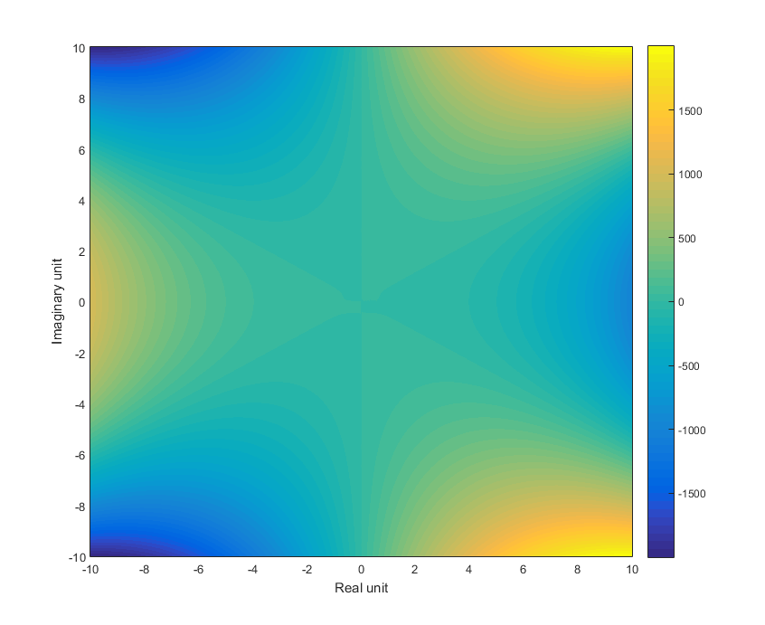
For plotting it's required to use a range of values. So, using x = a + b*i:

[a,b] = meshgrid(-10:0.1:10); %// creates two grids
ComplexValue = a+1i*b;        %// get a single, complex valued grid
CompFun = @(x)(- real(x.^3) + imag((10 + x.*1i)./(- 100.*x.^2 + x.*5i + 20))); %// add dots for element wise calculation
result = CompFun(ComplexValue); %// get results
pcolor(a,b,result) %// plot
shading interp %// remove grid borders by interpolation
colorbar %// add colour scale
ylabel 'Imaginary unit'
xlabel 'Real unit'

I did have to add dots (i.e. element wise multiplication) to your equation to make it work.

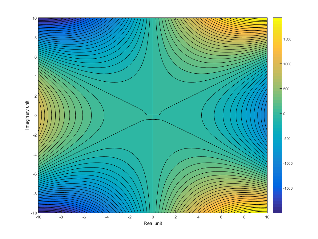
Additionally with the contourf as suggested in the comment by @AndrasDeak:

figure
contourf(a,b,result,51) %// plots with 51 contour levels
colorbar

I used a meshgrid of -10:0.01:10 here for more resolution:

If you are reluctant to hand-copy the solution to add the element wise multiplication dots, you can resort to loops:

grid = -10:0.1:10;
result(numel(grid),numel(grid))=0; %// initialise output grid
for a = 1:numel(grid)
    for b = 1:numel(grid)
        x = grid(a)+1i*grid(b);
        result(a,b) = ImaginaryPart(x);
    end
end

This delivers the same result, but with pros and cons both. It's slower than matrix-multiplication, i.e. than adding dots to your equation, but it does not require manipulating the output by hand.

Streamlet

Consider using a contourf instead/as well, with a lot of levels: zeroes are clearly visible then. – Placable

@LuisMendo here it is in jet, specially for you: i.imgur.com/QQijOZb.png – Streamlet

@Streamlet This should be a good illustration of what "perceptually uniform" means and why people don't like jet. It's the Comic Sans of color maps! – Berwick