Smoothing out a curve

Question

I have two lists of data points:

list_x = [-10, -9, -8, -7, -6, -5, -4, -3, -2, -1, 0, 1, 2, 3, 4, 5, 6, 7, 8, 9, 10, 11, 12, 13, 14, 15, 16, 17, 18, 19, 20, 21, 22, 23, 24, 25, 26, 27, 28, 29, 30, 31, 32, 33, 34, 35, 36, 37, 38, 39, 40, 41, 42, 43, 44, 45, 46, 47, 48, 49]
list_y = [1, 1, 1, 2, 2, 2, 2, 3, 3, 3, 4, 4, 5, 5, 5, 5, 5, 5, 5, 5, 5, 5, 5, 5, 5, 5, 4, 4, 4, 4, 3, 3, 3, 3, 3, 3, 2, 2, 2, 2, 2, 1, 1, 1, 1, 1, 1, 1, 1, 1, 1, 1, 1, 1, 1, 1, 1, 1, 1, 1]

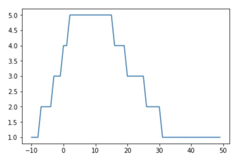
When I plot them, the graph will look like this:

import matplotlib.pyplot as plt
plt.plot(list_x, list_y)
plt.show()

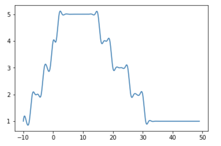
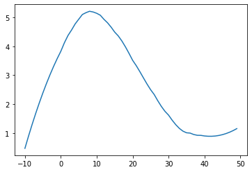
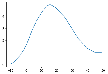
Based on these datapoints, is there a way to make the graph that looks like the one below and get its graph equation?

===========================================================

I have tried using the solution from here, and it produces a graph that is not smooth.

from scipy.interpolate import spline
import numpy as np

list_x_new = np.linspace(min(list_x), max(list_x), 1000)
list_y_smooth = spline(list_x, list_y, list_x_new)

plt.plot(list_x_new, list_y_smooth)
plt.show() 

Lens

Answer 1

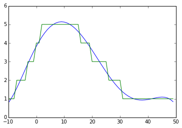
One easy option that echoes the suggestion from Davis Herring would be to use a polynomial approximation for the data

import numpy as np
import matplotlib.pyplot as plt

plt.figure()
poly = np.polyfit(list_x,list_y,5)
poly_y = np.poly1d(poly)(list_x)
plt.plot(list_x,poly_y)
plt.plot(list_x,list_y)
plt.show()

You would notice the oscillation at the right end of the plot that is not present in the original data which is an artifact of polynomial approximation.

Spline interpolation as suggested above by Davis is another good option. Varying the smoothness parameter s you can achieve different balance between smoothness and distance to the original data.

from scipy.interpolate import splrep, splev

plt.figure()
bspl = splrep(list_x,list_y,s=5)
bspl_y = splev(list_x,bspl)
plt.plot(list_x,list_y)
plt.plot(list_x,bspl_y)
plt.show()

Speakeasy

spline is now depricated. this answer describes the new usage with BSpline: https://mcmap.net/q/136287/-plot-smooth-line-with-pyplot – Syringe

I had issues implementing the seemingly newer BSpline. It could not handle None values and the curves were not as smooth as with spline. Likely my fault, but there is also no warning of splrep, splev being deprecated. Could it be that they are different from the deprecated spline? – Hearten

Could it be that BSpline is what is done manually in the script at the bottom? At least it works, has no warning of being deprecated, and is assigned to bspl which seems like an abbreviation of BSpline. – Hearten

Answer 2

Here are 3 more curve smoothing options:

1. Savitzky-Golay filter
2. LOWESS smoother
3. IIR filter

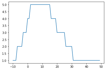
But first, recreate the original plot:

import matplotlib.pyplot as plt

list_x = [-10, -9, -8, -7, -6, -5, -4, -3, -2, -1, 0, 1, 2, 3, 4, 5, 6, 7, 8, 9, 10, 11, 12, 13, 14, 15, 16, 17, 18, 19, 20, 21, 22, 23, 24, 25, 26, 27, 28, 29, 30, 31, 32, 33, 34, 35, 36, 37, 38, 39, 40, 41, 42, 43, 44, 45, 46, 47, 48, 49]
list_y = [1, 1, 1, 2, 2, 2, 2, 3, 3, 3, 4, 4, 5, 5, 5, 5, 5, 5, 5, 5, 5, 5, 5, 5, 5, 5, 4, 4, 4, 4, 3, 3, 3, 3, 3, 3, 2, 2, 2, 2, 2, 1, 1, 1, 1, 1, 1, 1, 1, 1, 1, 1, 1, 1, 1, 1, 1, 1, 1, 1]

plt.plot(list_x, list_y)
plt.show()

---

1. Savitzky-Golay filter from scipy

The Savitzky-Golay technique fits subsets (windows) of adjacent points to low order polynomials using least squares.

How to apply the Savitzky-Golay filter:

from scipy.signal import savgol_filter

window = 21
order = 2
y_sf = savgol_filter(list_y, window, order)
plt.plot(list_x, y_sf)
plt.show()

The window and order parameters mean this filter is quite adaptable.

Read more about using this filter in the scipy documentation.

---

2. LOWESS smoother from statsmodels

LOWESS (locally weighted scatterplot smoothing) is a local regression method. In my experience it is simple to tune and often gives great results.

How to apply the LOWESS smoother:

import statsmodels.api as sm

y_lowess = sm.nonparametric.lowess(list_y, list_x, frac = 0.30)  # 30 % lowess smoothing

plt.plot(y_lowess[:, 0], y_lowess[:, 1])
plt.show()

It may be possible to improve the approximation by varying the frac parameter, which is the fraction of the data used when estimating each y value. Increase the frac value to increase the amount of smoothing. The frac value must be between 0 and 1.

Further details on statsmodels lowess usage.

---

3. IIR filter from scipy

After application of the lfilter:

from scipy.signal import lfilter

n = 15             # larger n gives smoother curves
b = [1.0 / n] * n  # numerator coefficients
a = 1              # denominator coefficient
y_lf = lfilter(b, a, list_y)

plt.plot(list_x, y_lf)
plt.show()

Check scipy lfilter documentation for implementation details regarding how numerator and denominator coefficients are used in the difference equations.

There are other filters in the scipy.signal package.

---

Care must be taken to avoid over-smoothing with all these approaches.

Additionally, some of these methods may have unexpected edge effects.

Gestapo

Answer 3

Because your data is approximate (i.e., it has been quantized), you want an approximating spline, not an interpolating spline.

Dave

While this link may answer the question, it is better to include the essential parts of the answer here and provide the link for reference. Link-only answers can become invalid if the linked page changes. - From Review – Dardani

@SimasJoneliunas: The requisite change to the code in the example is trivial, and duplicating SciPy’s documentation is a bit different from summarizing some random blog post. Meanwhile, the worked example that might have been useful was coopted by the other answer within minutes, so there’s no point now. – Dave