Calculate the modes in a multimodal distribution in R

Question

I have measured the body heights of all my children. When I plot all heights along an axis of lengths, this is what the result looks like:

Every red (boys) or violet (girls) tick is one child. If two children have the same body height (in millimetres), the ticks get stacked. Currently there are seven children with the same body height. (The height and width of the ticks is meaningless. They have been scaled to be visible.)

As you can see, the different heights are not evenly distributed along the axis, but cluster around certain values.

A histrogram and density plot of the data looks like this (with the two density estimates plotted following this answer):

As you can see, this is a multimodal distribution.

How do I calculate the modes (in R)?

---

Here is the raw data for you to play with:

mm <- c(418, 527, 540, 553, 554, 558, 613, 630, 634, 636, 645, 648, 708, 714, 715, 725, 806, 807, 822, 823, 836, 837, 855, 903, 908, 910, 911, 913, 915, 923, 935, 945, 955, 957, 958, 1003, 1006, 1015, 1021, 1021, 1022, 1034, 1043, 1048, 1051, 1054, 1058, 1100, 1102, 1103, 1117, 1125, 1134, 1138, 1145, 1146, 1150, 1152, 1210, 1211, 1213, 1223, 1226, 1334)

Pluralism

I think I got confused. Do you want to find the mode of mm? It is not a multimodal vector because the mode is 1021. Do you need any prior calculations using mm? – Raffarty

@Raffarty See en.wikipedia.org/wiki/Multimodal_distribution Simplified: What I want are the summits of the density curve in my question. – Pluralism

That's a lot of children. How big is your harem? – Cru

@ChuckD. Interesting. It took 5 hours for someone to comment on this :-) – Pluralism

A small number of observations drawn from a unimodal distribution will frequently look like this: (e.g., set.seed(6); hist(rnorm(64))), and a procedure to "find the modes" is ill-defined as there are many ways this could be done... – Hoptoad

Answer 1

I constructed something on my own using your mm data.

First let's plot the density of mm in order to visualise the modes:

plot(density(mm))

So, we can see there are 2 modes in this distribution. One around 600 and one around 1000. Let's see how to find them.

In order to find the mode indices I made this function:

find_modes<- function(x) {
  modes <- NULL
  for ( i in 2:(length(x)-1) ){
    if ( (x[i] > x[i-1]) & (x[i] > x[i+1]) ) {
      modes <- c(modes,i)
    }
  }
  if ( length(modes) == 0 ) {
    modes = 'This is a monotonic distribution'
  }
  return(modes)
}

Let's try it on our density:

mymodes_indices <- find_modes(density(mm)$y) #you need to try it on the y axis

Now mymodes_indices contains the indices of our modes i.e.:

> density(mm)$y[mymodes_indices]  #just to confirm that those are the correct
[1] 0.0008946929 0.0017766183

> density(mm)$x[mymodes_indices] #the actual modes
[1]  660.2941 1024.9067

Hope it helps!

Raffarty

This solution is highly dependent on the smoothing parameters and the underlying distribution and is not a general approach to this problem and will find "modes" in noise set.seed(6); find_modes(density(runif(64))$y) – Hoptoad

Answer 2

I modified the answer of Jeffrey Evans in Peak of the kernel density estimation to be allowed to modify the bw parameter and accordingly get more or less peaks. It is necessary for other cases, which will produce many peaks with the accepted answer. The parameter signifi allows handling ties.

library(dplyr)
library(tidyr)
get.modes2 <- function(x,adjust,signifi,from,to) {  
  den <- density(x, kernel=c("gaussian"),adjust=adjust,from=from,to=to)
  den.s <- smooth.spline(den$x, den$y, all.knots=TRUE, spar=0.1)
  s.1 <- predict(den.s, den.s$x, deriv=1)
  s.0 <- predict(den.s, den.s$x, deriv=0)
  den.sign <- sign(s.1$y)
  a<-c(1,1+which(diff(den.sign)!=0))
  b<-rle(den.sign)$values
  df<-data.frame(a,b)
  df = df[which(df$b %in% -1),]
  modes<-s.1$x[df$a]
  density<-s.0$y[df$a]
  df2<-data.frame(modes,density)
  df2$sig<-signif(df2$density,signifi)
  df2<-df2[with(df2, order(-sig)), ] 
  #print(df2)
  df<-as.data.frame(df2 %>% 
                      mutate(m = min_rank(desc(sig)) ) %>% #, count = sum(n)) %>% 
                      group_by(m) %>% 
                      summarize(a = paste(format(round(modes,2),nsmall=2), collapse = ',')) %>%
                      spread(m, a, sep = ''))
  colnames(df)<-paste0("m",1:length(colnames(df)))
  print(df)
}
mm <- c(418, 527, 540, 553, 554, 558, 613, 630, 634, 636, 645, 648, 708, 714, 715, 725, 806, 807, 822, 823, 836, 837, 855, 903, 908, 910, 911, 913, 915, 923, 935, 945, 955, 957, 958, 1003, 1006, 1015, 1021, 1021, 1022, 1034, 1043, 1048, 1051, 1054, 1058, 1100, 1102, 1103, 1117, 1125, 1134, 1138, 1145, 1146, 1150, 1152, 1210, 1211, 1213, 1223, 1226, 1334)
mmdf<-data.frame(mm=mm)
library(ggplot2)
#0.25 defines the number of peaks.
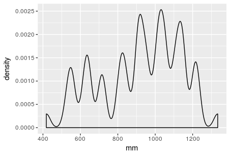
ggplot(mmdf,aes(mm)) + geom_density(adjust=0.25) + xlim((min(mm)-1),(max(mm)+1) )
#2 defines ties
modes<-get.modes2(mm,adjust=0.25,2,min(mm)-1,max(mm)+1)
#       m1     m2      m3            m4      m5     m6     m7              m8
#1 1031.40 921.81 1133.79 636.17,826.60 1216.43 548.14 715.22  418.80,1335.00

Lyte

Answer 3

This is the motivation of the "multimode" package.

Identifying modes is not as straightforward as simply checking when the direction of the "histogram curve" (or kernel density estimate) changes. Very crudely, we probably want to exclude very small peaks that might be down to noise. Setting a "bandwidth" parameter allows us to specify the scale at which a peak is attributed to "noise" rather than "signal".

The full statistical process, including multiple approaches to determining how many nodes are present, is described in the (open access) paper describing the package. Concisely, we can calculate the number and position of modes using:

mm <- c(418, 527, 540, 553, 554, 558, 613, 630, 634, 636, 645, 648, 708, 714, 715, 725, 806, 807, 822, 823, 836, 837, 855, 903, 908, 910, 911, 913, 915, 923, 935, 945, 955, 957, 958, 1003, 1006, 1015, 1021, 1021, 1022, 1034, 1043, 1048, 1051, 1054, 1058, 1100, 1102, 1103, 1117, 1125, 1134, 1138, 1145, 1146, 1150, 1152, 1210, 1211, 1213, 1223, 1226, 1334)

# Select an appropriate bandwidth. Here we use a "rule of thumb" method
bandwidth <- bw.nrd0(mm) 

# Other methods, e.g. bw.ucv(), will identify different bandwidths as optimal
# Consequently the number (and position) of modes may differ too

# Methods implemented in multimode are documented at ?bw.nrd

# Calculate number of modes
n <- nmodes(mm, bw = bandwidth)

# Calculate location of these modes
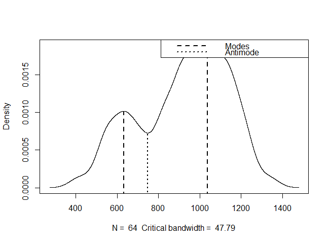
loc <- locmodes(mm, mod0 = n, display = TRUE)
# Remove `, display = TRUE` if you don't want to see the KDE
loc

Locations of modes are odd values in loc; even values are anti-modes (i.e. valley bottoms). Extract the locations of just the modes with:

modes <- loc$locations[seq(from = 1, by = 2, length.out = n)]

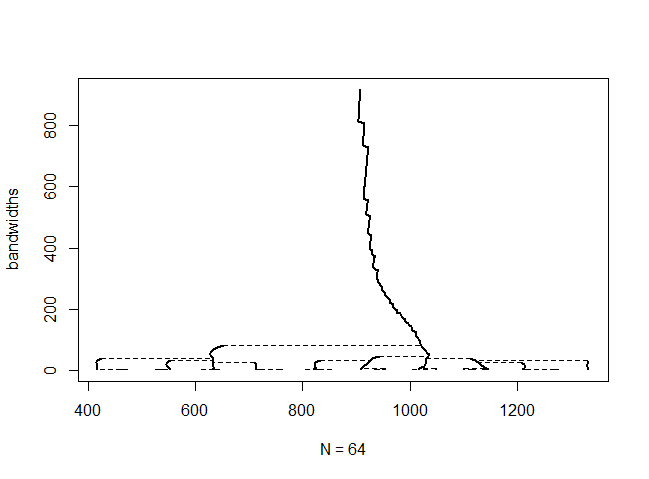
We can view how the number (and position) of modes varies with bandwidth using:

modetree(mm)

Arlettaarlette