Comparing survival at specific time points

Question

I have a following survival data

library(survival)
data(pbc)

#model to be plotted and analyzed, convert time to years
fit <- survfit(Surv(time/365.25, status) ~ edema, data = pbc)

#visualize overall survival Kaplan-Meier curve
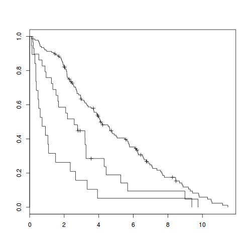
plot(fit)

Here is how the resulting Kaplan-Meier plot looks like

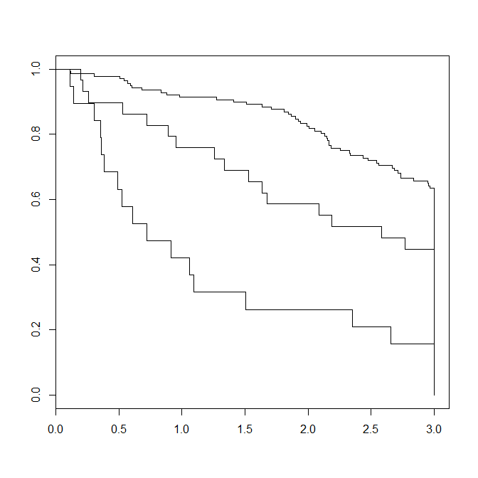
I am further calculating survival at 1, 2, 3 years in this manner:

>     summary(fit,times=c(1,2,3))

Call: survfit(formula = Surv(time/365.25, status) ~ edema, data = pbc)

232 observations deleted due to missingness 
                edema=0 
 time n.risk n.event survival std.err lower 95% CI upper 95% CI
    1    126      12    0.913  0.0240        0.867        0.961
    2    112      12    0.825  0.0325        0.764        0.891
    3     80      26    0.627  0.0420        0.550        0.714

                edema=0.5 
 time n.risk n.event survival std.err lower 95% CI upper 95% CI
    1     22       7    0.759  0.0795        0.618        0.932
    2     17       5    0.586  0.0915        0.432        0.796
    3     11       4    0.448  0.0923        0.299        0.671

                edema=1 
 time n.risk n.event survival std.err lower 95% CI upper 95% CI
    1      8      11    0.421  0.1133       0.2485        0.713
    2      5       3    0.263  0.1010       0.1240        0.558
    3      3       2    0.158  0.0837       0.0559        0.446

As you can see, the resulting output shows me 95% confidence intervals between different levels of edema but no actual p values. Whether confidence intervals overlap or not, I still get a pretty good idea whether survival at these time points are signifiantly different or not, but I would like to have exact p values. How can I do that?

Extine

I don't think you should and especially should not be asking for the use of an exact method. P-values would be more appropriate for the overall tests of differences between curves. – Typewriter

@42 there are situations where point survival is important and literature has many examples of it. Of course, P value for the overall difference is very important but I already have it. – Extine

Have you seen the lecture notes available here:biostat.wisc.edu/pub/chappell/641/notes.week7and8and9/…? As described in the linked document, there are multiple ways to accomplish this. – Picul

Surely it might be interesting to calculate p-values at a specific time, but that's not what you asked. You asked for an indiscriminate calculation of multiple values with no indication that you understood the statistics involved. – Typewriter

One approach would be to stop the follow-up at the time you are interested in. Let's say you're interested in 5-year disease-free survival (assuming that is clinically or biologically relevant); then you just focus on that part of the curve, and the follow-up is finished after the first 5 years (although you have longer follow-up data available; you don't use it). Calculating a log-rank test for this data set will result in a P-value that corresponds with differences in the 5-year survival rate. – Chisholm

Answer 1

Your question is 'are x-year survival rates different for the different categories of edema'.

For example, if you're interested in 3-year survival rates; you only need to focus on that portion of the curve (first 3 years of follow-up), as shown in the figure. The follow-up time for patients that are still alive after 3 years is set to 3 years (i.e., maximum follow-up time in this analysis):pbc$time[pbc$time > 3*365.25] <- 3*365.25.

Calculating a log-rank test using coxph in the package 'survival' (same package you are already using in your analysis) for this data set will provide you the P-value that says whether survival at three years is different between the three groups (highly significant in this example). You can also use the same model to generate P-values and hazard ratios for the association of edema with cause-specific survival.

Chisholm

thank you, it is a workaround and not necessarily a "timepoint" survival but still helpful. – Extine

I would disagree with the answer. Cox regression and logrank test (which are different tests, not one!) compare the curves on the whole time interval 0-3 years. But here we need to compare survival probabilities at 3 years, not survival probabilities on the whole interval! – Madame

Answer 2

I think the following code does what you are looking for:

library(survival)
data(pbc)

#model to be plotted and analyzed, convert time to years
fit <- survfit(Surv(time/365.25, status) ~ edema, data = pbc)

#visualize overall survival Kaplan-Meier curve
plot(fit)

threeYr <- summary(fit,times=3)

#difference in survival at 3 years between edema=0 and edemo=1 (for example) is
threeYr$surv[1] - threeYr$surv[3]
#the standard error of this is
diffSE <- sqrt(threeYr$std.err[3]^2 + threeYr$std.err[1]^2)
#a 95% CI for the diff is
threeYr$surv[1] - threeYr$surv[3] - 1.96 *diffSE
threeYr$surv[1] - threeYr$surv[3] + 1.96 *diffSE
#a z-test test statistic is
zStat <- (threeYr$surv[1] - threeYr$surv[3])/diffSE
#and a two-sided p-value testing that the diff. is 0 is
2*pnorm(abs(zStat), lower.tail=FALSE)

Alternatively one could make the comparison by estimating the risk ratio or odds ratio based on the estimated probabilities, and perform the inference/test on the log risk ratio or log odds ratio scale. In general I would expect this to perform better (in terms of test size and confidence interval coverage) since the normal approximation will be better on these scales than on the risk difference scale.

Scopula