TLDR

I have been trying to fit a simple neural network on MNIST, and it works for a small debugging setup, but when I bring it over to a subset of MNIST, it trains super fast and the gradient is close to 0 very quickly, but then it outputs the same value for any given input and the final cost is quite high. I had been trying to purposefully overfit to make sure it is in fact working but it will not do so on MNIST suggesting a deep problem in the setup. I have checked my backpropagation implementation using gradient checking and it seems to match up, so not sure where the error lies, or what to work on now!

Many thanks for any help you can offer, I've been struggling to fix this!

Explanation

I have been trying to make a neural network in Numpy, based on this explanation: http://ufldl.stanford.edu/wiki/index.php/Neural_Networks http://ufldl.stanford.edu/wiki/index.php/Backpropagation_Algorithm

Backpropagation seems to match gradient checking:

Backpropagation: [ 0.01168585,  0.06629858, -0.00112408, -0.00642625, -0.01339408,
   -0.07580145,  0.00285868,  0.01628148,  0.00365659,  0.0208475 ,
    0.11194151,  0.16696139,  0.10999967,  0.13873069,  0.13049299,
   -0.09012582, -0.1344335 , -0.08857648, -0.11168955, -0.10506167]
Gradient Checking: [-0.01168585 -0.06629858  0.00112408  0.00642625  0.01339408  
    0.07580145 -0.00285868 -0.01628148 -0.00365659 -0.0208475  
   -0.11194151 -0.16696139 -0.10999967 -0.13873069 -0.13049299  
    0.09012582  0.1344335   0.08857648  0.11168955  0.10506167]

And when I train on this simple debug setup:

a is a neural net w/ 2 inputs -> 5 hidden -> 2 outputs, and learning rate 0.5
a.gradDesc(np.array([[0.1,0.9],[0.2,0.8]]),np.array([[0,1],[0,1]]))
ie. x1 = [0.1, 0.9] and y1 = [0,1]

I get these lovely training curves

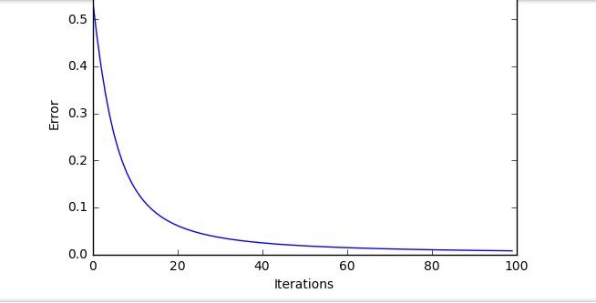
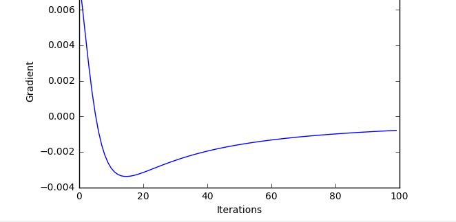
Admittedly this is clearly a dumbed down, very easy function to fit. However as soon as I bring it over to MNIST, with this setup:

    # Number of input, hidden and ouput nodes
    # Input = 28 x 28 pixels
    input_nodes=784
    # Arbitrary number of hidden nodes, experiment to improve
    hidden_nodes=200
    # Output = one of the digits [0,1,2,3,4,5,6,7,8,9]
    output_nodes=10

    # Learning rate
    learning_rate=0.4

    # Regularisation parameter
    lambd=0.0

With this setup run on the code below, for 100 iterations, it does seem to train at first then just "flat lines" quite quickly and doesnt achieve a very good model:

Initial ===== Cost (unregularised):  2.09203670985  /// Cost (regularised):      2.09203670985    Mean Gradient:  0.0321241229793
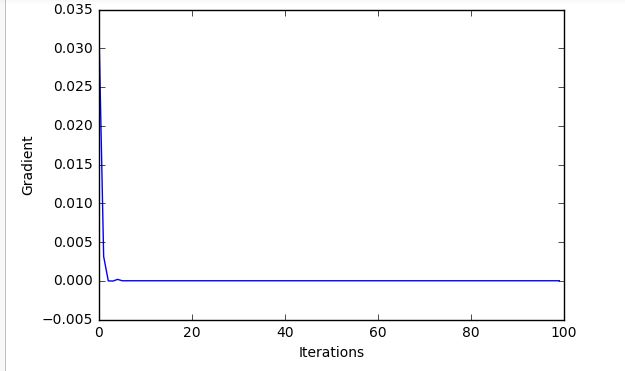
Iteration  100  Cost (unregularised):  0.980999805477   /// Cost (regularised):  0.980999805477    Mean Gradient:  -5.29639499854e-09
TRAINED IN  26.45932364463806

This then gives really poor test accuracy and predicts the same output, even when tested with all inputs being 0.1 or all 0.9 I just get the same output (although precisely which number it outputs varies depending on initial random weights):

Test accuracy:  8.92
Targets    2  2  1  7  2  2  0  2  3  
Hypothesis 5  5  5  5  5  5  5  5  5

And the curves for the MNIST Training:

Code dump:

# Import dependencies
import numpy as np
import time
import csv
import matplotlib.pyplot
import random
import math

# Read in training data
with open('MNIST/mnist_train_100.csv') as file:
    train_data=np.array([list(map(int,line.strip().split(','))) for line in file.readlines()])


# In[197]:

# Plot a sample of training data to visualise
displayData(train_data[:,1:], 25)


# In[198]:

# Read in test data
with open('MNIST/mnist_test.csv') as file:
    test_data=np.array([list(map(int,line.strip().split(','))) for line in file.readlines()])

# Main neural network class
class neuralNetwork:
    # Define the architecture
    def __init__(self, i, h, o, lr, lda):
        # Number of nodes in each layer
        self.i=i
        self.h=h
        self.o=o
        # Learning rate
        self.lr=lr
        # Lambda for regularisation
        self.lda=lda
        
        # Randomly initialise the parameters, input-> hidden and hidden-> output
        self.ih=np.random.normal(0.0,pow(self.h,-0.5),(self.h,self.i))
        self.ho=np.random.normal(0.0,pow(self.o,-0.5),(self.o,self.h))
   
    def predict(self, X):
        # GET HYPOTHESIS ESTIMATES/ OUTPUTS
        # Add bias node x(0)=1 for all training examples, X is now m x n+1
        # Then compute activation to hidden node
        z2=np.dot(X,self.ih.T) + 1
        #print(a1.shape)
        a2=sigmoid(z2)
        #print(ha)
        # Add bias node h(0)=1 for all training examples, H is now m x h+1
        # Then compute activation to output node
        z3=np.dot(a2,self.ho.T) + 1
        h=sigmoid(z3)
        outputs=np.argmax(h.T,axis=0)
        
        return outputs

    def backprop (self, X, y):
        try:
            m = X.shape[0]
        except:
            m=1

        # GET HYPOTHESIS ESTIMATES/ OUTPUTS
        # Add bias node x(0)=1 for all training examples, X is now m x n+1
        # Then compute activation to hidden node
        z2=np.dot(X,self.ih.T)
        #print(a1.shape)
        a2=sigmoid(z2)
        #print(ha)
        # Add bias node h(0)=1 for all training examples, H is now m x h+1
        # Then compute activation to output node
        z3=np.dot(a2,self.ho.T)
        h=sigmoid(z3)

        # Compute error/ cost for this setup (unregularised and regularise)
        costReg=self.costFunc(h,y)
        costUn=self.costFuncReg(h,y)

        # Output error term
        d3=-(y-h)*sigmoidGradient(z3)

        # Hidden error term
        d2=np.dot(d3,self.ho)*sigmoidGradient(z2)

        # Partial derivatives for weights
        D2=np.dot(d3.T,a2)
        D1=np.dot(d2.T,X)

        # Partial derivatives of theta with regularisation
        T2Grad=(D2/m)+(self.lda/m)*(self.ho)
        T1Grad=(D1/m)+(self.lda/m)*(self.ih)

        # Update weights
        # Hidden layer (weights 1)
        self.ih-=self.lr*(((D1)/m) + (self.lda/m)*self.ih)
        # Output layer (weights 2)
        self.ho-=self.lr*(((D2)/m) + (self.lda/m)*self.ho)

        # Unroll gradients to one long vector
        grad=np.concatenate(((T1Grad).ravel(),(T2Grad).ravel()))

        return costReg, costUn, grad
 
    def backpropIter (self, X, y):
        try:
            m = X.shape[0]
        except:
            m=1
        
        # GET HYPOTHESIS ESTIMATES/ OUTPUTS
        # Add bias node x(0)=1 for all training examples, X is now m x n+1
        # Then compute activation to hidden node
        z2=np.dot(X,self.ih.T)
        #print(a1.shape)
        a2=sigmoid(z2)
        #print(ha)
        # Add bias node h(0)=1 for all training examples, H is now m x h+1
        # Then compute activation to output node
        z3=np.dot(a2,self.ho.T)
        h=sigmoid(z3)
        
        # Compute error/ cost for this setup (unregularised and regularise)
        costUn=self.costFunc(h,y)
        costReg=self.costFuncReg(h,y)
        
        gradW1=np.zeros(self.ih.shape)
        gradW2=np.zeros(self.ho.shape)
        for i in range(m):
            delta3 = -(y[i,:]-h[i,:])*sigmoidGradient(z3[i,:])
            delta2 = np.dot(self.ho.T,delta3)*sigmoidGradient(z2[i,:])
            
            gradW2= gradW2 + np.outer(delta3,a2[i,:])
            gradW1 = gradW1 + np.outer(delta2,X[i,:])

        # Update weights
        # Hidden layer (weights 1)
        #self.ih-=self.lr*(((gradW1)/m) + (self.lda/m)*self.ih)
        # Output layer (weights 2)
        #self.ho-=self.lr*(((gradW2)/m) + (self.lda/m)*self.ho)

        # Unroll gradients to one long vector
        grad=np.concatenate(((gradW1).ravel(),(gradW2).ravel()))
        
        return costUn, costReg, grad
    
    def gradDesc(self, X, y):
        # Backpropagate to get updates
        cost,costreg,grad=self.backpropIter(X,y)

        # Unroll parameters
        deltaW1=np.reshape(grad[0:self.h*self.i],(self.h,self.i))
        deltaW2=np.reshape(grad[self.h*self.i:],(self.o,self.h))
        
        # m = no. training examples
        m=X.shape[0]
        #print (self.ih)
        self.ih -= self.lr * ((deltaW1))#/m) + (self.lda * self.ih)) 
        self.ho -= self.lr * ((deltaW2))#/m) + (self.lda * self.ho)) 
        #print(deltaW1)
        #print(self.ih)
        return cost,costreg,grad
        
    
    # Gradient checking to compute the gradient numerically to debug backpropagation
    def gradCheck(self, X, y):
        # Unroll theta
        theta=np.concatenate(((self.ih).ravel(),(self.ho).ravel()))
        # perturb will add and subtract epsilon, numgrad will store answers
        perturb=np.zeros(len(theta))
        numgrad=np.zeros(len(theta))
        # epsilon, e is a small number
        e = 0.00001
        # Loop over all theta
        for i in range(len(theta)):
            # Perturb is zeros with one index being e
            perturb[i]=e
            loss1=self.costFuncGradientCheck(theta-perturb, X, y)
            loss2=self.costFuncGradientCheck(theta+perturb, X, y)
            # Compute numerical gradient and update vectors
            numgrad[i]=(loss1-loss2)/(2*e)
            perturb[i]=0
        return numgrad
        
    def costFuncGradientCheck(self,theta,X,y):
        T1=np.reshape(theta[0:self.h*self.i],(self.h,self.i))
        T2=np.reshape(theta[self.h*self.i:],(self.o,self.h))
        m=X.shape[0]
        # GET HYPOTHESIS ESTIMATES/ OUTPUTS
        # Compute activation to hidden node
        z2=np.dot(X,T1.T)
        a2=sigmoid(z2)
        # Compute activation to output node
        z3=np.dot(a2,T2.T)
        h=sigmoid(z3)
        
        cost=self.costFunc(h, y)
        return cost #+ ((self.lda/2)*(np.sum(pow(T1,2)) + np.sum(pow(T2,2))))
    
    def costFunc(self, h, y):
        m=h.shape[0]
        return np.sum(pow((h-y),2))/m
        
    def costFuncReg(self, h, y):
        cost=self.costFunc(h, y)
        return cost #+ ((self.lda/2)*(np.sum(pow(self.ih,2)) + np.sum(pow(self.ho,2))))
        
# Helper functions to compute sigmoid and gradient for an input number or matrix
def sigmoid(Z):
    return np.divide(1,np.add(1,np.exp(-Z)))
def sigmoidGradient(Z):
    return sigmoid(Z)*(1-sigmoid(Z))

# Pre=processing helper functions
# Normalise data to 0.1-1 as 0 inputs kills the weights and changes
def scaleDataVec(data):
    return (np.asfarray(data[1:]) / 255.0 * 0.99) + 0.1

def scaleData(data):
    return (np.asfarray(data[:,1:]) / 255.0 * 0.99) + 0.1

# DISPLAY DATA
# plot_data will be what to plot, num_ex must be a square number of how many examples to plot, random examples will then be plotted
def displayData(plot_data, num_ex, rand=1):
    if rand==0:
        data=plot_data
    else:
        rand_indexes=random.sample(range(plot_data.shape[0]),num_ex)
        data=plot_data[rand_indexes,:]
    # Useful variables, m= no. train ex, n= no. features
    m=data.shape[0]
    n=data.shape[1]
    # Shape for one example
    example_width=math.ceil(math.sqrt(n))
    example_height=math.ceil(n/example_width)
    # No. of items to display
    display_rows=math.floor(math.sqrt(m))
    display_cols=math.ceil(m/display_rows)
    # Padding between images
    pad=1
    # Setup blank display
    display_array = -np.ones((pad + display_rows * (example_height + pad), (pad + display_cols * (example_width + pad))))
    curr_ex=0
    for i in range(1,display_rows+1):
        for j in range(1,display_cols+1):
            if curr_ex>m:
                break
            # Max value of this patch
            max_val=max(abs(data[curr_ex, :]))
            display_array[pad + (j-1) * (example_height + pad) : j*(example_height+1), pad + (i-1) * (example_width + pad) :                           i*(example_width+1)] = data[curr_ex, :].reshape(example_height, example_width)/max_val
            curr_ex+=1

    matplotlib.pyplot.imshow(display_array, cmap='Greys', interpolation='None')


# In[312]:

a=neuralNetwork(2,5,2,0.5,0.0)
print(a.backpropIter(np.array([[0.1,0.9],[0.2,0.8]]),np.array([[0,1],[0,1]])))
print(a.gradCheck(np.array([[0.1,0.9],[0.2,0.8]]),np.array([[0,1],[0,1]])))
D=[]
C=[]
for i in range(100):
    c,b,d=a.gradDesc(np.array([[0.1,0.9],[0.2,0.8]]),np.array([[0,1],[0,1]]))
    C.append(c)
    D.append(np.mean(d))
    #print(c)
    
print(a.predict(np.array([[0.1,0.9]])))
# Debugging plot
matplotlib.pyplot.figure()
matplotlib.pyplot.plot(C)
matplotlib.pyplot.ylabel("Error")
matplotlib.pyplot.xlabel("Iterations")
matplotlib.pyplot.figure()
matplotlib.pyplot.plot(D)
matplotlib.pyplot.ylabel("Gradient")
matplotlib.pyplot.xlabel("Iterations")
#print(J)


# In[313]:

# Class instance

# Number of input, hidden and ouput nodes
# Input = 28 x 28 pixels
input_nodes=784
# Arbitrary number of hidden nodes, experiment to improve
hidden_nodes=200
# Output = one of the digits [0,1,2,3,4,5,6,7,8,9]
output_nodes=10

# Learning rate
learning_rate=0.4

# Regularisation parameter
lambd=0.0

# Create instance of Nnet class
nn=neuralNetwork(input_nodes,hidden_nodes,output_nodes,learning_rate,lambd)


# In[314]:

time1=time.time()
# Scale inputs
inputs=scaleData(train_data)
# 0.01-0.99 range as the sigmoid function can't reach 0 or 1, 0.01 for all except 0.99 for target
targets=(np.identity(output_nodes)*0.98)[train_data[:,0],:]+0.01
J=[]
JR=[]
Grad=[]
iterations=100
for i in range(iterations):
    j,jr,grad=nn.gradDesc(inputs, targets)
    grad=np.mean(grad)
    if i == 0:
        print("Initial ===== Cost (unregularised): ", j, "\t///", "Cost (regularised): ",jr,"   Mean Gradient: ",grad)
    print("\r", end="")
    print("Iteration ", i+1, "\tCost (unregularised): ", j, "\t///", "Cost (regularised): ", jr,"   Mean Gradient: ",grad,end="")
    J.append(j)
    JR.append(jr)
    Grad.append(grad)
time2 = time.time()
print ("\nTRAINED IN ",time2-time1)


# In[315]:

# Debugging plot
matplotlib.pyplot.figure()
matplotlib.pyplot.plot(J)
matplotlib.pyplot.plot(JR)
matplotlib.pyplot.ylabel("Error")
matplotlib.pyplot.xlabel("Iterations")
matplotlib.pyplot.figure()
matplotlib.pyplot.plot(Grad)
matplotlib.pyplot.ylabel("Gradient")
matplotlib.pyplot.xlabel("Iterations")
#print(J)


# In[316]:

# Scale inputs
inputs=scaleData(test_data)
# 0.01-0.99 range as the sigmoid function can't reach 0 or 1, 0.01 for all except 0.99 for target
targets=test_data[:,0]
h=nn.predict(inputs)
score=[]
targ=[]
hyp=[]
for i,line in enumerate(targets):
    if line == h[i]:
        score.append(1)
    else:
        score.append(0)
    hyp.append(h[i])
    targ.append(line)
print("Test accuracy: ", sum(score)/len(score)*100)
indexes=random.sample(range(len(hyp)),9)
print("Targets    ",end="")
for j in indexes:
    print (targ[j]," ",end="")
print("\nHypothesis ",end="")
for j in indexes:
    print (hyp[j]," ",end="")
displayData(test_data[indexes, 1:], 9, rand=0)


# In[277]:

nn.predict(0.9*np.ones((784,)))

Edit 1

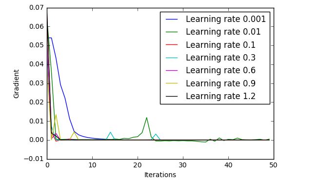
Suggested to use different learning rates, but unfortunately, they all come out with similar results, here are the plots for 30 iterations, using the MNIST 100 subset:

Concretely, here are the figures that they start and end with:

    Initial ===== Cost (unregularised):  4.07208963507  /// Cost (regularised):  4.07208963507    Mean Gradient:  0.0540251381858
    Iteration  50   Cost (unregularised):  0.613310215166   /// Cost (regularised):  0.613310215166    Mean Gradient:  -0.000133981500849Initial ===== Cost (unregularised):  5.67535252616     /// Cost (regularised):  5.67535252616    Mean Gradient:  0.0644797515914
    Iteration  50   Cost (unregularised):  0.381080434935   /// Cost (regularised):  0.381080434935    Mean Gradient:  0.000427866902699Initial ===== Cost (unregularised):  3.54658422176  /// Cost (regularised):  3.54658422176    Mean Gradient:  0.0672211732868
    Iteration  50   Cost (unregularised):  0.981    /// Cost (regularised):  0.981    Mean Gradient:  2.34515341943e-20Initial ===== Cost (unregularised):  4.05269658215   /// Cost (regularised):  4.05269658215    Mean Gradient:  0.0469666696193
    Iteration  50   Cost (unregularised):  0.980999999999   /// Cost (regularised):  0.980999999999    Mean Gradient:  -1.0582706063e-14Initial ===== Cost (unregularised):  2.40881492228  /// Cost (regularised):  2.40881492228    Mean Gradient:  0.0516056901574
    Iteration  50   Cost (unregularised):  1.74539997258    /// Cost (regularised):  1.74539997258    Mean Gradient:  1.01955789614e-09Initial ===== Cost (unregularised):  2.58498876008   /// Cost (regularised):  2.58498876008    Mean Gradient:  0.0388768685257
    Iteration  3    Cost (unregularised):  1.72520399313    /// Cost (regularised):  1.72520399313    Mean Gradient:  0.0134040908157
    Iteration  50   Cost (unregularised):  0.981    /// Cost (regularised):  0.981    Mean Gradient:  -4.49319474346e-43Initial ===== Cost (unregularised):  4.40141352357  /// Cost (regularised):  4.40141352357    Mean Gradient:  0.0689167742968
    Iteration  50   Cost (unregularised):  0.981    /// Cost (regularised):  0.981    Mean Gradient:  -1.01563966458e-22

A learning rate of 0.01, quite low, has the best outcome, but exploring learning rates in this region, I only came out with 30-40% accuracy, a big improvement on the 8% or even 0% that I had seen previously, but not really what it should be achieving!

Edit 2

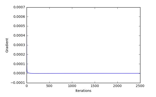
I've now finished and added a backpropagation function optimized for matrices rather than the iterative formula, and so now I can run it on large epochs/ iterations without painfully slow. So the "backprop" function of the class matches with gradient check (in fact it is 1/2 the size but I think that is a problem in gradient check, so we'll leave that bc it should not matter proportionally and I have tried with adding in divisions to solve this). With large numbers of epochs I achieved a much better accuracy, but still there seems to be a problem, as when I have previously programmed a slightly different style of simple 3 layer neural network a part of a book, on the same dataset csvs, I get a much better training result. Here are some plots and data for large epochs.

Looks good but, we still have a pretty poor test set accuracy, and this is for 2,500 runs through the dataset, should be getting a good result with much less!

    Test accuracy:  61.150000000000006
    Targets    6  9  8  2  2  2  4  3  8  
    Hypothesis 6  9  8  4  7  1  4  3  8

Edit 3, what dataset?

http://makeyourownneuralnetwork.blogspot.co.uk/2015/03/the-mnist-dataset-of-handwitten-digits.html?m=1

Used train.csv and test.csv to try with more data and no better just takes longer so been using the subset train_100 and test_10 while I debug.

Edit 4

Seems to learn something after a very large number of epochs (like 14,000), as the whole dataset is used in the backprop function (not backpropiter) each loop is effectively an epoch, and with a ridiculous amount of epochs on the subset of 100 train and 10 test samples, the test accuracy is quite good. However with this small a sample this could easily be due to just chance and even then it's only 70% percent not what you'd be aiming for even on the small dataset. But it does show that it seems to be learning, I am trying parameters very extensively to rule that out.