ggplot2 - adding secondary y-axis on top of a plot
Asked Answered
H

1

3

For a publication I need to add a second y-axis to an existing plot. I've come across a means of how to do this (https://rpubs.com/kohske/dual_axis_in_ggplot2). However, I don't really understand much of the coding. I cannot find a way to make it so that the right y-axis shows too, and only not the top border. What am I missing in my coding? This is my dummy data:

df1 <- structure(list(month = structure(1:12, .Label = c("Apr", "Aug", 
"Dec", "Feb", "Jan", "Jul", "Jun", "Mar", "May", "Nov", "Oct", 
"Sep"), class = "factor"), RI = c(0.52, 0.115, 0.636666666666667, 
0.807, 0.66625, 0.34, 0.143333333333333, 0.58375, 0.173333333333333, 
0.5, 0.13, 0), sd = c(0.327566787083184, 0.162634559672906, 0.299555225848813, 
0.172887246493199, 0.293010848165827, 0.480832611206852, 0.222785397486759, 
0.381610777775321, 0.219393102292058, 0.3, 0.183847763108502, 
0)), .Names = c("month", "RI", "sd"), class = "data.frame", row.names = c(NA, 
-12L))

df2<-structure(list(month = structure(c(5L, 4L, 8L, 1L, 9L, 7L, 6L, 
2L, 12L, 11L, 10L, 3L), .Label = c("Apr", "Aug", "Dec", "Feb", 
"Jan", "Jul", "Jun", "Mar", "May", "Nov", "Oct", "Sep"), class = "factor"), 
    temp = c(25, 25, 25, 25, 25, 25, 25, 25, 25, 25, 25, 25)), .Names = c("month", 
"temp"), row.names = c(NA, -12L), class = "data.frame")

library(ggplot2)
library(gtable)
library(grid)

p1 <-
  ggplot(data = df1, aes(x=month,y=RI)) + 
  geom_errorbar(aes(ymin=0,ymax=RI+sd),width=0.2,color="grey") +
  geom_bar(width=0.5,stat="identity",position=position_dodge()) +
  scale_y_continuous(limits=c(0,1),expand = c(0,0)) +  scale_x_discrete(limits=c("Jan","Feb","Mar","Apr","May","Jun","Jul","Aug","Sep","Oct","Nov","Dec")) +
  theme_bw(base_size = 12, base_family = "Helvetica") + 
  theme(panel.grid = element_blank()) +
  theme( # Increase size of axis lines
    axis.line.x = element_line(size = .7, color = "black"),
    axis.line.y = element_line(size = .7, color = "black"),
    panel.border = element_blank())

p2 <- 
  ggplot(data=df2) +
  geom_line(linetype="dashed",size=0.5,aes(x=month,y=temp,fullrange=T,group=1)) +
  scale_y_continuous(name = "Water temperature (°C)", limits = c(20,32)) +
  scale_x_discrete(limits=c("Jan","Feb","Mar","Apr","May","Jun","Jul","Aug","Sep","Oct","Nov","Dec")) +
  theme_bw(base_size = 12, base_family = "Helvetica") + 
  theme(panel.grid = element_blank()) +
  theme( # Increase size of axis lines
    axis.line.x = element_line(size = .7, color = "black"),
    axis.line.y = element_line(size = .7, color = "black"),
    panel.border = element_blank())


# Get the ggplot grobs
g1 <- ggplotGrob(p1)
g2 <- ggplotGrob(p2)

# Get the location of the plot panel in g1.
# These are used later when transformed elements of g2 are put back into g1
pp <- c(subset(g1$layout, name == "panel", se = t:r))

# ggplot contains many labels that are themselves complex grob; 
# usually a text grob surrounded by margins.
# When moving the grobs from, say, the left to the right of a plot,
# make sure the margins and the justifications are swapped around.
# The function below does the swapping.
# Taken from the cowplot package:
# https://github.com/wilkelab/cowplot/blob/master/R/switch_axis.R 

hinvert_title_grob <- function(grob){

  # Swap the widths
  widths <- grob$widths
  grob$widths[1] <- widths[3]
  grob$widths[3] <- widths[1]
  grob$vp[[1]]$layout$widths[1] <- widths[3]
  grob$vp[[1]]$layout$widths[3] <- widths[1]

  # Fix the justification
  grob$children[[1]]$hjust <- 1 - grob$children[[1]]$hjust 
  grob$children[[1]]$vjust <- 1 - grob$children[[1]]$vjust 
  grob$children[[1]]$x <- unit(1, "npc") - grob$children[[1]]$x
  grob
}

# Get the y axis title from g2 - "Elevation (ft)" 
index <- which(g2$layout$name == "ylab") # Which grob contains the y axis title?
ylab <- g2$grobs[[index]]                # Extract that grob
ylab <- hinvert_title_grob(ylab)         # Swap margins and fix justifications

# Put the transformed label on the right side of g1
g1 <- gtable_add_cols(g1, g2$widths[g2$layout[index, ]$l], pp$r)
g1 <- gtable_add_grob(g1, ylab, pp$t, pp$r + 1, pp$b, pp$r + 1, clip = "off", name = "ylab-r")

# Get the y axis from g2 (axis line, tick marks, and tick mark labels)
index <- which(g2$layout$name == "axis-l")  # Which grob
yaxis <- g2$grobs[[index]]                  # Extract the grob

# yaxis is a complex of grobs containing the axis line, the tick marks, and the tick mark labels.
# The relevant grobs are contained in axis$children:
#   axis$children[[1]] contains the axis line;
#   axis$children[[2]] contains the tick marks and tick mark labels.

# First, move the axis line to the left
yaxis$children[[1]]$x <- unit.c(unit(0, "npc"), unit(0, "npc"))

# Second, swap tick marks and tick mark labels
ticks <- yaxis$children[[2]]
ticks$widths <- rev(ticks$widths)
ticks$grobs <- rev(ticks$grobs)

# Third, move the tick marks
ticks$grobs[[1]]$x <- ticks$grobs[[1]]$x - unit(1, "npc") + unit(3, "pt")

# Fourth, swap margins and fix justifications for the tick mark labels
ticks$grobs[[2]] <- hinvert_title_grob(ticks$grobs[[2]])

# Fifth, put ticks back into yaxis
yaxis$children[[2]] <- ticks

# Put the transformed yaxis on the right side of g1
g1 <- gtable_add_cols(g1, g2$widths[g2$layout[index, ]$l], pp$r)
g1 <- gtable_add_grob(g1, yaxis, pp$t, pp$r + 1, pp$b, pp$r + 1, clip = "off", name = "axis-r")

# Draw it
grid.newpage()
grid.draw(g1)
Hut answered 20/4, 2016 at 20:48 Comment(4)
Your best option is not to do it. Try faceting or plotting both variables against each other and labelling date with an aesthetic like colour or shape.Electrotherapeutics
add a working example and the version you are using. axis.line is being ignored for me. and also the ?theme examples do not work. try axis.line.x/axis.line.y until the authors decide to fix itBreeding
if you don't understand the code, it's probably safer not to use it (especially since it's very likely to break in future versions of ggplot2). That being said, if all you need for now is the missing vertical line you could add an annotate("vline") at x=Inf.Reincarnate
Well, maybe it's best to not use it if you don't know how it works, but I am struggling to find alternatives.. @baptiste: your solution seems to work for now. thanksHut
R
6

Updated to ggplot2 v 2.2.1, but it is easier to use sec.axis - see here

Original

From ggplot2 version 2.1.0, the business of moving axes around became a lot more complex, the reason being that the labels became complex grobs containing text grobs and margins. (There is also a bug with axis.line. A temporary workaround is to set the x-axis and y-axis lines separately.)

The solution draws on older solutions that work on older ggplot versions, and on the cowplot function for copying and moving axes. But be aware that the solution could break with future versions of ggplot2.

I've used made up data from an old solution. The example shows two scales measuring the same thing - feet and metres.

library(ggplot2) # v 2.2.1
library(gtable)  # v 0.2.0
library(grid)

df <- data.frame(Day = c(1:365), Elevation = sin(seq(0, 2 * pi, 2 * pi / 364)) * 10 + 100)

p1 <- ggplot(data = df) + 
        geom_line(aes(x = Day,y = Elevation)) + 
        scale_y_continuous(name = "Elevation (m)", limits = c(75, 125)) +
        theme_bw(base_size = 12, base_family = "Helvetica") + 
        theme(panel.grid = element_blank()) +
        theme( # Increase size of axis lines
          axis.line.x = element_line(size = .7, color = "black"),
          axis.line.y = element_line(size = .7, color = "black"),
          panel.border = element_blank())


p2 <- ggplot(data = df)+
        geom_line(aes(x = Day, y = Elevation))+
        scale_y_continuous(name = "Elevation (ft)", limits = c(75, 125),           
          breaks=c(80, 90, 100, 110, 120),
          labels=c("262", "295", "328", "361", "394")) +
        theme_bw(base_size = 12, base_family = "Helvetica") + 
        theme(panel.grid = element_blank()) +
        theme( # Increase size of axis lines
          axis.line.x = element_line(size = .7, color = "black"),
          axis.line.y = element_line(size = .7, color = "black"),
          panel.border = element_blank())


# Get the ggplot grobs
g1 <- ggplotGrob(p1)
g2 <- ggplotGrob(p2)

# Get the location of the plot panel in g1.
# These are used later when transformed elements of g2 are put back into g1
pp <- c(subset(g1$layout, name == "panel", se = t:r))

# ggplot contains many labels that are themselves complex grob; 
# usually a text grob surrounded by margins.
# When moving the grobs from, say, the left to the right of a plot,
# make sure the margins and the justifications are swapped around.
# The function below does the swapping.
# Taken from the cowplot package:
# https://github.com/wilkelab/cowplot/blob/master/R/switch_axis.R 

hinvert_title_grob <- function(grob){

  # Swap the widths
  widths <- grob$widths
  grob$widths[1] <- widths[3]
  grob$widths[3] <- widths[1]
  grob$vp[[1]]$layout$widths[1] <- widths[3]
  grob$vp[[1]]$layout$widths[3] <- widths[1]

  # Fix the justification
  grob$children[[1]]$hjust <- 1 - grob$children[[1]]$hjust 
  grob$children[[1]]$vjust <- 1 - grob$children[[1]]$vjust 
  grob$children[[1]]$x <- unit(1, "npc") - grob$children[[1]]$x
  grob
}

# Get the y axis title from g2 - "Elevation (ft)" 
index <- which(g2$layout$name == "ylab-l") # Which grob contains the y axis title?
ylab <- g2$grobs[[index]]                # Extract that grob
ylab <- hinvert_title_grob(ylab)         # Swap margins and fix justifications

# Put the transformed label on the right side of g1
g1 <- gtable_add_cols(g1, g2$widths[g2$layout[index, ]$l], pp$r)
g1 <- gtable_add_grob(g1, ylab, pp$t, pp$r + 1, pp$b, pp$r + 1, clip = "off", name = "ylab-r")

# Get the y axis from g2 (axis line, tick marks, and tick mark labels)
index <- which(g2$layout$name == "axis-l")  # Which grob
yaxis <- g2$grobs[[index]]                  # Extract the grob

# yaxis is a complex of grobs containing the axis line, the tick marks, and the tick mark labels.
# The relevant grobs are contained in axis$children:
#   axis$children[[1]] contains the axis line;
#   axis$children[[2]] contains the tick marks and tick mark labels.

# First, move the axis line to the left
yaxis$children[[1]]$x <- unit.c(unit(0, "npc"), unit(0, "npc"))

# Second, swap tick marks and tick mark labels
ticks <- yaxis$children[[2]]
ticks$widths <- rev(ticks$widths)
ticks$grobs <- rev(ticks$grobs)

# Third, move the tick marks
ticks$grobs[[1]]$x <- ticks$grobs[[1]]$x - unit(1, "npc") + unit(3, "pt")

# Fourth, swap margins and fix justifications for the tick mark labels
ticks$grobs[[2]] <- hinvert_title_grob(ticks$grobs[[2]])

# Fifth, put ticks back into yaxis
yaxis$children[[2]] <- ticks

# Put the transformed yaxis on the right side of g1
g1 <- gtable_add_cols(g1, g2$widths[g2$layout[index, ]$l], pp$r)
g1 <- gtable_add_grob(g1, yaxis, pp$t, pp$r + 1, pp$b, pp$r + 1, clip = "off", name = "axis-r")

# Draw it
grid.newpage()
grid.draw(g1)
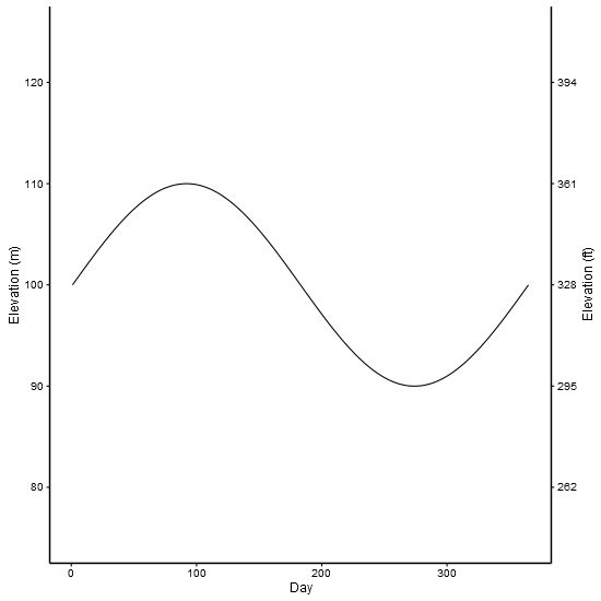
enter image description here


Second example shows how to include two different scale. But be aware that there is much to be criticised here: separate y scales, and dynamite plots

df1 <- structure(list(month = structure(1:12, .Label = c("Apr", "Aug", 
"Dec", "Feb", "Jan", "Jul", "Jun", "Mar", "May", "Nov", "Oct", 
"Sep"), class = "factor"), RI = c(0.52, 0.115, 0.636666666666667, 
0.807, 0.66625, 0.34, 0.143333333333333, 0.58375, 0.173333333333333, 
0.5, 0.13, 0), sd = c(0.327566787083184, 0.162634559672906, 0.299555225848813, 
0.172887246493199, 0.293010848165827, 0.480832611206852, 0.222785397486759, 
0.381610777775321, 0.219393102292058, 0.3, 0.183847763108502, 
0)), .Names = c("month", "RI", "sd"), class = "data.frame", row.names = c(NA, 
-12L))

df2<-structure(list(month = structure(c(5L, 4L, 8L, 1L, 9L, 7L, 6L, 
2L, 12L, 11L, 10L, 3L), .Label = c("Apr", "Aug", "Dec", "Feb", 
"Jan", "Jul", "Jun", "Mar", "May", "Nov", "Oct", "Sep"), class = "factor"), 
    temp = c(25, 25, 25, 25, 25, 25, 25, 25, 25, 25, 25, 25)), .Names = c("month", 
"temp"), row.names = c(NA, -12L), class = "data.frame")

library(ggplot2)
library(gtable)
library(grid)

p1 <-
  ggplot(data = df1, aes(x=month,y=RI)) + 
  geom_errorbar(aes(ymin=0,ymax=RI+sd),width=0.2,color="grey") +
  geom_bar(width=0.5,stat="identity",position=position_dodge(), fill = "grey") +
  scale_y_continuous(limits=c(0,1),expand = c(0,0)) +  scale_x_discrete(limits=c("Jan","Feb","Mar","Apr","May","Jun","Jul","Aug","Sep","Oct","Nov","Dec")) +
  theme_bw(base_size = 12, base_family = "Helvetica") + 
  theme(panel.grid = element_blank()) +
  theme( # Increase size of axis lines
    axis.line.x = element_line(size = .7, color = "black"),
    axis.line.y = element_line(size = .7, color = "black"),
    panel.border = element_blank())

# Note transparent background for the second plot
p2 <- 
  ggplot(data=df2) +
  geom_line(linetype="dashed",size=0.5,aes(x=month,y=temp,group=1)) +
  scale_y_continuous(name = "Water temperature (°C)", limits = c(20,32)) +
  scale_x_discrete(limits=c("Jan","Feb","Mar","Apr","May","Jun","Jul","Aug","Sep","Oct","Nov","Dec")) +
  theme_bw(base_size = 12, base_family = "Helvetica") + 
  theme(panel.grid = element_blank()) +
  theme( # Increase size of axis lines
    axis.line.x = element_line(size = .7, color = "black"),
    axis.line.y = element_line(size = .7, color = "black"),
    panel.border = element_blank(),
    panel.background = element_rect(fill = "transparent"))

# Get the ggplot grobs
g1 <- ggplotGrob(p1)
g2 <- ggplotGrob(p2)


# Get the location of the plot panel in g1.
# These are used later when transformed elements of g2 are put back into g1
pp <- c(subset(g1$layout, name == "panel", se = t:r))

# Overlap panel for second plot on that of the first plot
g1 <- gtable_add_grob(g1, g2$grobs[[which(g2$layout$name == "panel")]], pp$t, pp$l, pp$b, pp$l)

# Then proceed as before:

# ggplot contains many labels that are themselves complex grob; 
# usually a text grob surrounded by margins.
# When moving the grobs from, say, the left to the right of a plot,
# Make sure the margins and the justifications are swapped around.
# The function below does the swapping.
# Taken from the cowplot package:
# https://github.com/wilkelab/cowplot/blob/master/R/switch_axis.R 

hinvert_title_grob <- function(grob){

  # Swap the widths
  widths <- grob$widths
  grob$widths[1] <- widths[3]
  grob$widths[3] <- widths[1]
  grob$vp[[1]]$layout$widths[1] <- widths[3]
  grob$vp[[1]]$layout$widths[3] <- widths[1]

  # Fix the justification
  grob$children[[1]]$hjust <- 1 - grob$children[[1]]$hjust 
  grob$children[[1]]$vjust <- 1 - grob$children[[1]]$vjust 
  grob$children[[1]]$x <- unit(1, "npc") - grob$children[[1]]$x
  grob
}

# Get the y axis title from g2
index <- which(g2$layout$name == "ylab-l") # Which grob contains the y axis title?
ylab <- g2$grobs[[index]]                # Extract that grob
ylab <- hinvert_title_grob(ylab)         # Swap margins and fix justifications

# Put the transformed label on the right side of g1
g1 <- gtable_add_cols(g1, g2$widths[g2$layout[index, ]$l], pp$r)
g1 <- gtable_add_grob(g1, ylab, pp$t, pp$r + 1, pp$b, pp$r + 1, clip = "off", name = "ylab-r")

# Get the y axis from g2 (axis line, tick marks, and tick mark labels)
index <- which(g2$layout$name == "axis-l")  # Which grob
yaxis <- g2$grobs[[index]]                  # Extract the grob

# yaxis is a complex of grobs containing the axis line, the tick marks, and the tick mark labels.
# The relevant grobs are contained in axis$children:
#   axis$children[[1]] contains the axis line;
#   axis$children[[2]] contains the tick marks and tick mark labels.

# First, move the axis line to the left
yaxis$children[[1]]$x <- unit.c(unit(0, "npc"), unit(0, "npc"))

# Second, swap tick marks and tick mark labels
ticks <- yaxis$children[[2]]
ticks$widths <- rev(ticks$widths)
ticks$grobs <- rev(ticks$grobs)

# Third, move the tick marks
ticks$grobs[[1]]$x <- ticks$grobs[[1]]$x - unit(1, "npc") + unit(3, "pt")

# Fourth, swap margins and fix justifications for the tick mark labels
ticks$grobs[[2]] <- hinvert_title_grob(ticks$grobs[[2]])

# Fifth, put ticks back into yaxis
yaxis$children[[2]] <- ticks

# Put the transformed yaxis on the right side of g1
g1 <- gtable_add_cols(g1, g2$widths[g2$layout[index, ]$l], pp$r)
g1 <- gtable_add_grob(g1, yaxis, pp$t, pp$r + 1, pp$b, pp$r + 1, clip = "off", name = "axis-r")

# Draw it
grid.newpage()
grid.draw(g1)
Rocray answered 21/4, 2016 at 3:53 Comment(8)
@Walter, credit goes to Claus Wilke, author of cowplot package.Rocray
@MvZB What versions of r, ggplot2, gtable are you running?Rocray
r v 3.2.1, ggplot v 2.1.0, gtable v 0.2.0. I just updated ggplot2, it seems to work now. Great, thanks.Hut
@SandyMuspratt: I tried to apply your code to my data set, with some additional coding, but for some reason p2 doesn't overlay on p1. Any suggestions what to change in my coding? I updated my OP. Thank youHut
@MvZB Without data, it's hard to say. I was dealing with equivalent measures - feet and metres - and hence no overlaying. It looks like you want two different measures: one for the bar charts, one for the lines. This is not advised (see bosek's advice above). But if you must, you need to decide which chart goes on top, make sure it has a transparent plot background, grab its plot panel, and overley the panel into the plot panel spot of the first plot. If you run into trouble, provide some data, and I'll have a go at it, but probably not today.Rocray
@SandyMuspratt I provided a reproducible example. I hope you can help me out. thanksHut
@MvZB See the second exampleRocray
@SandyMuspratt, thank you, the dynamite plots is an eye opener.Hut

© 2022 - 2024 — McMap. All rights reserved.