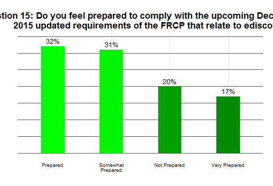
Gradient fill for geom_bar scaled relative to each bar and not mapped to a variable

Question

My goal is to reproduce this plot, and my problem is reproducing the gradient fill in each bar.

ADDED after COMMENT The good comment of @PavoDive directs us to a question that basically says "You can't do it with ggplot2 and furthermore it is a bad idea even if you could do it." Agreed as to it being a poor graphical choice, but for didactic purposes I wanted to re-create the original and then show improvements. So, is there a programming solution nevertheless?

With the data that follows the ggplot code I have gotten close, other than the consistent gradient coloring that is the same for each bar (and the tiny tick marks). But my efforts result in bars that are filled to match the y value, while in the original plot each bar is filled with the same pattern. How do I achieve that effect?

ggplot(df, aes(x = x, y = y, fill = y)) +
  geom_hline(yintercept = seq(0, .35, .05), color = "grey30", size = 0.5, linetype = "solid") +
  geom_bar(stat = "identity", width = 0.4) +
  scale_fill_gradient(low='green4', high='green1', guide = FALSE) +
  theme(legend.position = "none") +
  theme_minimal() +
  geom_text(data = df, aes(label = scales::percent(y), vjust = -.5)) +
  theme(axis.text.y = element_blank()) +
  theme(axis.ticks = element_blank()) +
  labs(y = "", x = "") +
  ggtitle("Question 15: Do you feel prepared to comply with the upcoming December
          2015 updated requirements of the FRCP that relate to ediscovery") +
  theme(plot.title = element_text(face = "bold", size = 18)) +
  theme(panel.border = element_blank())

Data

df <- data.frame(x = c("Prepared", "Somewhat\nprepared", "Not prepared", "Very prepared"),
                 y = c(.32, .31, .20, .17))
df$x <- factor(df$x, levels = c("Prepared", "Somewhat\nPrepared", "Not Prepared", "Very Prepared"))

Doyle

possible duplicate of Gradient Fill in Bar Graph – Arabian

@PavoDive: the SO question you link to (and thank you for doing so) does not give an answer because "The gradient you describe adds nothing to the graphic, and would be a prime example of "chart junk". That kind of thing is made difficult, nigh on impossible in ggplot on purpose, because it is widely considered to be a bad idea" I agree with the commenter but I am still trying to reproduce the plot so I can blog about how to improve it. – Doyle

I see your point. Then, I suggest you make an edit and actually reference that post, so people coming to yours will know that you know and avoid "editorializing" over the convenience of doing it, and stick to the programming challenge of actually doing it. If you don't, then you'll get answers in the same line of the post I referenced as a duplicate – Arabian

Wow, that made a drastic change! I'm going from "flag" to "upvote"! And the wonderful answer by @nongkrong showed that it is indeed possible (even if unnecessary or even bad practice). – Arabian

Answer 1

Here is an option, using geom_path with a scaled y to color by instead of bars. This creates some new data (dat), sequences from 0 to each df$y value (length 100 here, in column dat$y). Then, a scaled version of each sequence is created (from 0 to 1), that is used as the color gradient (called dat$scaled). The scaling is done by simply dividing each sequence by its maximum value.

## Make the data for geom_path
mat <- mapply(seq, 0, df$y, MoreArgs = list(length=100))                         # make sequences 0 to each df$y
dat <- stack(data.frame(lapply(split(mat, col(mat)), function(x) x/tail(x,1))))  # scale each, and reshape
dat$x <- rep(df$x, each=100)                                                     # add the x-factors
dat$y <- stack(as.data.frame(mat))[,1]                                           # add the unscaled column
names(dat)[1] <- "scaled"                                                        # rename

## Make the plot
ggplot(dat, aes(x, y, color=scaled)) +                                           # use different data
  ## *** removed some code here ***
  geom_hline(yintercept = seq(0, .35, .05), color = "grey30", size = 0.5, linetype = "solid") +
  theme(legend.position = "none") +
  theme_minimal() +
  geom_text(data = df, aes(label = scales::percent(y), vjust = -.5), color="black") +
  theme(axis.text.y = element_blank()) +
  theme(axis.ticks = element_blank()) +
  labs(y = "", x = "") +
  ggtitle("Question 15: Do you feel prepared to comply with the upcoming December
          2015 updated requirements of the FRCP that relate to ediscovery") +
            theme(plot.title = element_text(face = "bold", size = 18)) +
            theme(panel.border = element_blank()) +
  ## *** Added this code ***            
  geom_path(lwd=20) +
  scale_color_continuous(low='green4', high='green1', guide=F)

Dowsabel

Wow! Would you mind adding some explanation for your code that creates mat and scaled color? – Doyle

Answer 2

This may be acheived with functions from package gridSVG. I use a stripped-down version of your example with only the most necessary parts for the actual problem:

# load additional packages
library(grid)
library(gridSVG)

# create a small data set
df <- data.frame(x = factor(1:3), y = 1:3)

# a basic bar plot to be modified
ggplot(data = df, aes(x = x, y = y)) +
  geom_bar(stat = "identity") 

# create a linear color gradient
cols <- linearGradient(col = c("green4", "green1"),
                       x0 = unit(0.5, "npc"), x1 = unit(0.5, "npc"))

# create a definition of a gradient fill
registerGradientFill(label = "cols", gradient = cols)

# list the names of grobs and look for the relevant geometry 
grid.ls()
# GRID.gTableParent.76
# ...snip...
#  panel.3-4-3-4
#    geom_rect.rect.2 # <~~~~ this is the grob! Note that the number may differ

# apply the gradient to each bar
grid.gradientFill("geom_rect.rect", label = rep("cols", length(unique(df$x))),
                  group = FALSE, grep = TRUE)

# generate SVG output from the grid graphics
grid.export("myplot.svg")

You find more gridSVG examples here, here, and here.

Lemcke

I think you needn't worry about the number 43, grep=TRUE should find it for you – Gasper

Forgot about the grep argument. Thanks for the reminder @baptiste! Edited. – Lemcke

This example does not work. The command grid.ls() does not list the grobs specified in your commented code. Perhaps the graphics device must be changed? – Rogers

@Rogers Thanks for the heads-up! Yes, the ggplot2 machinery has undergone some major changes since I posted my answer. I will try to update the code when I get time. Cheers. – Lemcke

Great long-term support @Henrik. this is why i love s.o. :-) – Rogers

Answer 3

Using ggplot2 >= 3.5.0 (and R >= 4.2.0) which adds support for gradient fills this can now more easily be achieved.

Similar to the approach by @Henrik this requires to create a gradient fill first using e.g. grid::linearGradient which could then be passed to the fill= argument of geom_bar:

library(ggplot2)

packageVersion("ggplot2")
#> [1] '3.5.0'

grad_ungroup <- grid::linearGradient(c("green4", "green1"), group = FALSE)

ggplot(df, aes(x = x, y = y, fill = y)) +
  geom_hline(
    yintercept = seq(0, .35, .05),
    color = "grey30", size = 0.5, linetype = "solid"
  ) +
  geom_bar(stat = "identity", width = 0.4, fill = grad_ungroup) +
  theme(legend.position = "none") +
  theme_minimal() +
  geom_text(data = df, aes(label = scales::percent(y), vjust = -.5)) +
  theme(axis.text.y = element_blank()) +
  theme(axis.ticks = element_blank()) +
  labs(y = "", x = "") +
  ggtitle("Question 15: Do you feel prepared to comply with the upcoming December
          2015 updated requirements of the FRCP that relate to ediscovery") +
  theme(plot.title = element_text(face = "bold", size = 18)) +
  theme(panel.border = element_blank())

Bugloss