How to fit a polynomial with some of the coefficients constrained?

Question

Using NumPy's polyfit (or something similar) is there an easy way to get a solution where one or more of the coefficients are constrained to a specific value?

For example, we could find the ordinary polynomial fitting using:

x = np.array([0.0, 1.0, 2.0, 3.0,  4.0,  5.0])
y = np.array([0.0, 0.8, 0.9, 0.1, -0.8, -1.0])
z = np.polyfit(x, y, 3)

yielding

array([ 0.08703704, -0.81349206,  1.69312169, -0.03968254])

But what if I wanted the best fit polynomial where the third coefficient (in the above case z[2]) was required to be 1? Or will I need to write the fitting from scratch?

Nopar

I think in this case you would be better off with scipy's curve_fit function or lmfit. – Hypercritical

As @Hypercritical said, use scipy.optimize.curve_fit() and use the bounds arg to set lower and upper bounds on independent variables. – Lonnie

Answer 1

In this case, I would use curve_fit or lmfit; I quickly show it for the first one.

import numpy as np
import matplotlib.pyplot as plt
from scipy.optimize import curve_fit

def func(x, a, b, c, d):
  return a + b * x + c * x ** 2 + d * x ** 3

x = np.array([0.0, 1.0, 2.0, 3.0,  4.0,  5.0])
y = np.array([0.0, 0.8, 0.9, 0.1, -0.8, -1.0])

print(np.polyfit(x, y, 3))

popt, _ = curve_fit(func, x, y)
print(popt)

popt_cons, _ = curve_fit(func, x, y, bounds=([-np.inf, 2, -np.inf, -np.inf], [np.inf, 2.001, np.inf, np.inf]))
print(popt_cons)

xnew = np.linspace(x[0], x[-1], 1000)

plt.plot(x, y, 'bo')
plt.plot(xnew, func(xnew, *popt), 'k-')
plt.plot(xnew, func(xnew, *popt_cons), 'r-')
plt.show()

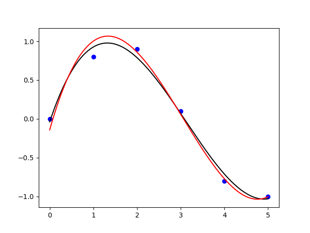
This will print:

[ 0.08703704 -0.81349206  1.69312169 -0.03968254]
[-0.03968254  1.69312169 -0.81349206  0.08703704]
[-0.14331349  2.         -0.95913556  0.10494372]

So in the unconstrained case, polyfit and curve_fit give identical results (just the order is different), in the constrained case, the fixed parameter is 2, as desired.

The plot looks then as follows:

In lmfit you can also choose whether a parameter should be fitted or not, so you can then also just set it to a desired value (check this answer).

Hypercritical

Answer 2

Sorry for the resurrection

..but I felt that this answer was missing.

To fit a polynomial we solve the following system of equations:

a0*x0^n + a1*x0^(n-1) .. + an*x0^0 = y0
a0*x1^n + a1*x1^(n-1) .. + an*x1^0 = y1
                 ...
a0*xm^n + a1*xm^(n-1) .. + an*xm^0 = ym

Which is a problem of the form V @ a = y

where "V" is a Vandermonde matrix:

[[x0^n  x0^(n-1)  1],
 [x1^n  x1^(n-1)  1],
        ...
 [xm^n  xm^(n-1)  1]]

"y" is a column vector holding the y-values:

[[y0],
 [y1],
  ...
 [ym]]

..and "a" is the column vector of coefficients that we are solving for:

[[a0],
 [a1],
  ...
 [an]]

This problem can be solved using linear least squares as follows:

import numpy as np

x = np.array([0.0, 1.0, 2.0, 3.0,  4.0,  5.0])
y = np.array([0.0, 0.8, 0.9, 0.1, -0.8, -1.0])

deg = 3
V = np.vander(x, deg + 1)
z, *_ = np.linalg.lstsq(V, y, rcond=None)

print(z)
# [ 0.08703704 -0.81349206  1.69312169 -0.03968254]

..which produces the same solution as the polyfit method:

z = np.polyfit(x, y, deg)

print(z)
# [ 0.08703704 -0.81349206  1.69312169 -0.03968254]

Instead we want a solution where a2 = 1

substituting a2 = 1 into the system of equations from the beginning of the answer, and then moving the corresponding term from the lhs to the rhs we get:

a0*x0^n + a1*x0^(n-1) + 1*x0^(n-2) .. + an*x0^0 = y0
a0*x1^n + a1*x1^(n-1) + 1*x0^(n-2) .. + an*x1^0 = y1
                 ...
a0*xm^n + a1*xm^(n-1) + 1*x0^(n-2) .. + an*xm^0 = ym

=>

a0*x0^n + a1*x0^(n-1) .. + an*x0^0 = y0 - 1*x0^(n-2)
a0*x1^n + a1*x1^(n-1) .. + an*x1^0 = y1 - 1*x0^(n-2)
                 ...
a0*xm^n + a1*xm^(n-1) .. + an*xm^0 = ym - 1*x0^(n-2)

This corresponds to removing column 2 from the Vandermonde matrix and subtracting it from the y-vector as follows:

y_ = y - V[:, 2]
V_ = np.delete(V, 2, axis=1)
z_, *_ = np.linalg.lstsq(V_, y_, rcond=None)
z_ = np.insert(z_, 2, 1)

print(z_)
# [ 0.04659264 -0.48453866  1.          0.19438046]

Notice that I inserted the 1 in the coefficient vector after solving the linear least-squares problem, we are no longer solving for a2 since we set it to 1 and removed it from the problem.

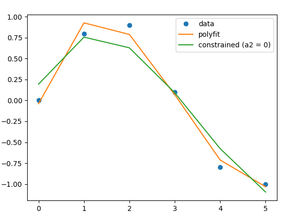
For completeness this is what the solution looks like when plotted:

and the complete code that I used:

import numpy as np

x = np.array([0.0, 1.0, 2.0, 3.0,  4.0,  5.0])
y = np.array([0.0, 0.8, 0.9, 0.1, -0.8, -1.0])

deg = 3
V = np.vander(x, deg + 1)
z, *_ = np.linalg.lstsq(V, y, rcond=None)

print(z)
# [ 0.08703704 -0.81349206  1.69312169 -0.03968254]

z = np.polyfit(x, y, deg)

print(z)
# [ 0.08703704 -0.81349206  1.69312169 -0.03968254]

y_ = y - V[:, 2]
V_ = np.delete(V, 2, axis=1)
z_, *_ = np.linalg.lstsq(V_, y_, rcond=None)
z_ = np.insert(z_, 2, 1)

print(z_)
# [ 0.04659264 -0.48453866  1.          0.19438046]

from matplotlib import pyplot as plt

plt.plot(x, y, 'o', label='data')
plt.plot(x, V @ z, label='polyfit')
plt.plot(x, V @ z_, label='constrained (a2 = 0)')

plt.legend()

plt.show()

Lohman

Answer 3

For completeness, with lmfit the solution would look like this:

import numpy as np
import matplotlib.pyplot as plt
from lmfit import Model

def func(x, a, b, c, d):
    return a + b * x + c * x ** 2 + d * x ** 3

x = np.array([0.0, 1.0, 2.0, 3.0,  4.0,  5.0])
y = np.array([0.0, 0.8, 0.9, 0.1, -0.8, -1.0])

pmodel = Model(func)
params = pmodel.make_params(a=1, b=2, c=1, d=1)

params['b'].vary = False 

result = pmodel.fit(y, params, x=x)

print(result.fit_report())

xnew = np.linspace(x[0], x[-1], 1000)
ynew = result.eval(x=xnew)

plt.plot(x, y, 'bo')
plt.plot(x, result.best_fit, 'k-')
plt.plot(xnew, ynew, 'r-')
plt.show()

which would print a comprehensive report, including uncertainties, correlations and fit statistics as:

[[Model]]
    Model(func)
[[Fit Statistics]]
    # fitting method   = leastsq
    # function evals   = 10
    # data points      = 6
    # variables        = 3
    chi-square         = 0.066
    reduced chi-square = 0.022
    Akaike info crit   = -21.089
    Bayesian info crit = -21.714
[[Variables]]
    a:  -0.14331348 +/- 0.109441 (76.37%) (init= 1)
    b:   2 (fixed)
    c:  -0.95913555 +/- 0.041516 (4.33%) (init= 1)
    d:   0.10494371 +/- 0.008231 (7.84%) (init= 1)
[[Correlations]] (unreported correlations are <  0.100)
    C(c, d)                      = -0.987
    C(a, c)                      = -0.695
    C(a, d)                      =  0.610

and produce a plot of

Note that lmfit.Model has many improvements over curve_fit, including automatically naming parameters based on function arguments, allowing any parameter to have bounds or simply be fixed without requiring nonsense like having upper and lower bounds that are almost equal. The key is that lmfit uses Parameter objects that have attributes instead of plain arrays of fitting variables. lmfit also supports mathematical constraints, composite models (eg, adding or multiplying models), and has superior reports.

Lowtension

This is great, especially the extended stats and the no-nonsense bounds! I'm bookmarking this post for future reference. – Lonnie

Answer 4

Here is a general way using scipy.optimize.curve_fit aiming to fix whatever the polynomial coefficients are desired.

import numpy as np
from scipy.optimize import curve_fit

def polyfit(x, y, deg, which=-1, to=0):
    """
    An extension of ``np.polyfit`` to fix values of the vector 
    of polynomial coefficients. By default, the last coefficient 
    (i.e., the constant term) is kept at zero.

    Parameters
    ----------
    x : array_like
        x-coordinates of the sample points.
    y : array_like
        y-coordinates of the sample points.
    deg : int
        Degree of the fitting polynomial.
    which : int or array_like, optional
        Indexes of the coefficients to remain fixed. By default, -1.
    to : float or array_like, optional
        Values of the fixed coefficients. By default, 0.

    Returns
    -------
    np.ndarray
        (deg + 1) polynomial coefficients.
    """
    p0 = np.polyfit(x, y, deg)

    # if which == None it is reduced to np.polyfit
    if which is None: 
        return p0
    
    # indexes of the coeffs being fitted
    which_not = np.delete(np.arange(deg + 1), which)
    
    # create the array of coeffs
    def _fill_p(p):
        p_ = np.empty(deg + 1)  # empty array
        p_[which] = to          # fill with custom coeffs
        p_[which_not] = p       # fill with `p`
        return p_

    # callback function for fitting
    def _polyfit(x, *p):
        p_ = _fill_p(p)
        return np.polyval(p_, x)

    # get the array of coeffs
    p0 = np.delete(p0, which)                # use `p0` as initial condition
    p, _ = curve_fit(_polyfit, x, y, p0=p0)  # fitting
    p = _fill_p(p)                           # merge fixed and no-fixed coeffs
    return p

Two simple examples on how to use the function above:

import matplotlib.pyplot as plt

# just create some fake data (a parabola)
np.random.seed(0)                               # seed to reproduce the example
deg = 2                                         # second order polynomial
p = np.random.randint(1, 5, size=deg+1)         # random vector of coefficients
x = np.linspace(0, 10, num=20)                  # fake data: x-array
y = np.polyval(p, x) + 1.5*np.random.randn(20)  # fake data: y-array
print(p)                                        # output:[1, 4, 2]

# fitting
p1 = polyfit(x, y, deg, which=2, to=p[2])        # case 1: last coeff is fixed
p2 = polyfit(x, y, deg, which=[1,2], to=p[1:3])  # case 2: last two coeffs are fixed
y1 = np.polyval(p1, x)                           # y-array for case 1
y2 = np.polyval(p2, x)                           # y-array for case 2
print(p1)                                        # output: [1.05, 3.67, 2.]
print(p2)                                        # output: [1.08, 4.,   2.]

# plotting
plt.plot(x, y, '.', label='fake data: y = p[0]*x**2 + p[1]*x + p[2]')
plt.plot(x, y1, label='p[2] fixed at 2')
plt.plot(x, y2, label='p[2] and p[1] fixed at [4, 2]')
plt.legend()
plt.show()

Aquino

Answer 5

Here is a way to do this using scipy.optimize.curve_fit:

First, let's recreate your example (as a sanity check):

import numpy as np
from scipy.optimize import curve_fit
​
def f(x, x3, x2, x1, x0):
    """this is the polynomial function"""
    return x0 + x1*x + x2*(x*x) + x3*(x*x*x)
​
popt, pcov = curve_fit(f, x, y)

print(popt)
#array([ 0.08703704, -0.81349206,  1.69312169, -0.03968254])

Which matches the values you get from np.polyfit().

Now adding the constraints for x1:

popt, pcov = curve_fit(
    f, 
    x,
    y,
    bounds = ([-np.inf, -np.inf, .999999999, -np.inf], [np.inf, np.inf, 1.0, np.inf])
)
print(popt)
#array([ 0.04659264, -0.48453866,  1.        ,  0.19438046])

I had to use .999999999 because the lower bound must be strictly less than the upper bound.

Alternatively, you could define your function with the constrained coefficient as a constant, and get the values for the other 3:

def f_new(x, x3, x2, x0):
    x1 = 1
    return x0 + x1*x + x2*(x*x) + x3*(x*x*x)
popt, pcov = curve_fit(f_new, x, y)
print(popt)
#array([ 0.04659264, -0.48453866,  0.19438046])

Lonnie