How to correctly interpret ggplot's stat_density2d

Question

My initial goal was to plot a population of individual points and then draw a convex hull enclosing 80% of that population centered on the mass of the population.

After trying a number of ideas, the best solution I came up with was to use ggplot's stat_density2d. While this works great for a qualitative analysis, I still need to indicate an 80% boundary. I started out looking for a way to outline the 80th percentile population boundary, but I can work with an 80% probability density boundary instead.

Here's where I'm looking for help. The bin parameter for kde2d (used by stat_density2d) is not clearly documented. If I set bin = 4 in the example below, am I correct in interpreting the central (green) region as containing a 25% probability mass and the combined yellow, red, and green areas as representing a 75% probability mass? If so, by changing the bin to = 5, would the area inscribed then equal an 80% probability mass?

set.seed(1)
n=100

df <- data.frame(x=rnorm(n, 0, 1), y=rnorm(n, 0, 1))

TestData <- ggplot (data = df) +
  stat_density2d(aes(x = x, y = y, fill = as.factor(..level..)), 
  bins=4, geom = "polygon", ) +
  geom_point(aes(x = x, y = y)) +
  scale_fill_manual(values = c("yellow","red","green","royalblue", "black"))

TestData

I repeated a number of test cases and manually counted the excluded points [would love to find a way to count them based on what ..level.. they were contained within] but given the random nature of the data (both my real data and the test data) the number of points outside of the stat_density2d area varied enough to warrant asking for help.

Summarizing, is there a practical means of drawing a polygon around the central 80% of the population of points in the data frame? Or, baring that, am I safe to use stat_density2d and set bin equal to 5 to produce an 80% probability mass?

---

Excellent answer from Bryan Hanson dispelling the fuzzy notion that I could pass an undocumented bin parameter in stat_density2d. The results looked close at values for bin around 4 to 6, but as he stated, the actual function is unknown and therefore not usable.

I used the HDRegionplot as provided in the accepted answer by DWin to solve my problem. To that, I added a center of gravity (COGravity) and point in polygon (pnt.in.poly) from the SDMTools package to complete the analysis.

library(MASS)
library(coda)
library(SDMTools)
library(emdbook)
library(ggplot2)


theme_set(theme_bw(16))
set.seed(1)
n=100

df <- data.frame(x=rnorm(n, 0, 1), y=rnorm(n, 0, 1))

HPDregionplot(mcmc(data.matrix(df)), prob=0.8)
with(df, points(x,y))
ContourLines <- as.data.frame(HPDregionplot(mcmc(data.matrix(df)), prob=0.8))
df$inpoly <- pnt.in.poly(df, ContourLines[, c("x", "y")])$pip

dp <- df[df$inpoly == 1,]
COG100 <- as.data.frame(t(COGravity(df$x, df$y)))
COG80 <- as.data.frame(t(COGravity(dp$x, dp$y)))

TestData <- ggplot (data = df) +
  stat_density2d(aes(x = x, y = y, fill = as.factor(..level..)), 
  bins=5, geom = "polygon", ) +
  geom_point(aes(x = x, y = y, colour = as.factor(inpoly)), alpha = 1) +
  geom_point(data=COG100, aes(COGx, COGy),colour="white",size=2, shape = 4) +
  geom_point(data=COG80, aes(COGx, COGy),colour="green",size=4, shape = 3) +
  geom_polygon(data = ContourLines, aes(x = x, y = y), color = "blue", fill = NA) +
  scale_fill_manual(values = c("yellow","red","green","royalblue", "brown", "black", "white", "black", "white","black")) +
  scale_colour_manual(values = c("red", "black"))
TestData 
nrow(dp)/nrow(df) # actual number of population members inscribed within the 80% probability polgyon

Battledore

Answer 1

HPDregionplot in package:emdbook is supposed to do that. It does use MASS::kde2d but it normalizes the result. It has the disadvantage to my mind that it requires an mcmc object.

library(MASS)
library(coda)
HPDregionplot(mcmc(data.matrix(df)), prob=0.8)
with(df, points(x,y))

Philipphilipa

Answer 2

Alright, let me start by saying I'm not entirely sure of this answer, and it's only a partial answer! There is no bin parameter for MASS::kde2d which is the function used by stat_density2d. Looking at the help page for kde2d and the code for it (seen simply by typing the function name in the console), I think the bin parameter is h (how these functions know to pass bin to h is not clear however). Following the help page, we see that if h is not provided, it is computed by MASS:bandwidth.nrd. The help page for that function says this:

# The function is currently defined as
function(x)
{
    r <- quantile(x, c(0.25, 0.75))
    h <- (r[2] - r[1])/1.34
    4 * 1.06 * min(sqrt(var(x)), h) * length(x)^(-1/5)
}

Based on this, I think the answer to your last question ("Am I safe...") is definitely no. r in the above function is what you need for your assumption to be safe, but it is clearly modified, so you are not safe. HTH.

Additional thought: Do you have any evidence that your code is using your bins argument? I'm wondering if it is being ignored. If so, try passing h in place of bins and see if it listens.

Cuneal

Answer 3

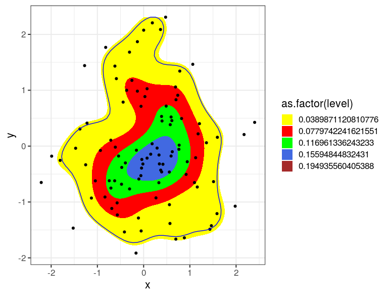
Building on the answer by 42, I've simplified HPDregionplot() to reduce dependencies and remove the requirement to work with mcmc-objects. The function works on a two-column data.frame and creates no intermediate plots. Note, however, that the this approach breaks as soon as grDevices::contourLines() return multiple contours.

hpd_contour <- function (x, n = 50, prob = 0.95, ...) {
  post1 <- MASS::kde2d(x[[1]], x[[2]], n = n, ...)

  dx <- diff(post1$x[1:2])
  dy <- diff(post1$y[1:2])
  sz <- sort(post1$z)
  c1 <- cumsum(sz) * dx * dy

  levels <- sapply(prob, function(x) {
    approx(c1, sz, xout = 1 - x)$y
  })

  as.data.frame(grDevices::contourLines(post1$x, post1$y, post1$z, levels = levels))
}

theme_set(theme_bw(16))
set.seed(1)
n=100

df <- data.frame(x=rnorm(n, 0, 1), y=rnorm(n, 0, 1))
ContourLines <- hpd_contour(df, prob=0.8)

ggplot(df, aes(x = x, y = y)) +
  stat_density2d(aes(fill = as.factor(..level..)), bins=5, geom = "polygon") +
  geom_point() +
  geom_polygon(data = ContourLines, color = "blue", fill = NA) +
  scale_fill_manual(values = c("yellow","red","green","royalblue", "brown", "black", "white", "black", "white","black")) +
  scale_colour_manual(values = c("red", "black"))

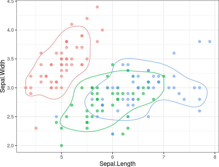
Moreover, the workflow now easily extends to grouped data.

ContourLines <- iris[, c("Species", "Sepal.Length", "Sepal.Width")] %>% 
  group_by(Species) %>% 
  do(hpd_contour(.[, c("Sepal.Length", "Sepal.Width")], prob=0.8))

ggplot(data = iris, aes(x = Sepal.Length, y = Sepal.Width, color = Species)) +
  geom_point(size = 3, alpha = 0.6) +
  geom_polygon(data = ContourLines, fill = NA) +
  guides(color = FALSE) +
  theme(plot.margin = margin())

Garibold

The bins argument seems to be fixed now. If you want to compute bins for each group, you need to compute them on normalised densities, see Claus WIlke's reply in this GitHub thread github.com/tidyverse/ggplot2/issues/4113 – Fumble