FFT on image with Python

Question

I have a problem with FFT implementation in Python. I have completely strange results. Ok so, I want to open image, get value of every pixel in RGB, then I need to use fft on it, and convert to image again.

My steps:

1) I'm opening image with PIL library in Python like this

from PIL import Image
im = Image.open("test.png")

2) I'm getting pixels

pixels = list(im.getdata())

3) I'm seperate every pixel to r,g,b values

for x in range(width):
    for y in range(height):
        r,g,b = pixels[x*width+y]
        red[x][y] = r
        green[x][y] = g
        blue[x][y] = b

4). Let's assume that I have one pixel (111,111,111). And use fft on all red values like this

red = np.fft.fft(red)

And then:

print (red[0][0], green[0][0], blue[0][0])

My output is:

(53866+0j) 111 111

It's completely wrong I think. My image is 64x64, and FFT from gimp is completely different. Actually, my FFT give me only arrays with huge values, thats why my output image is black.

Do you have any idea where is problem?

[EDIT]

I've changed as suggested to

red= np.fft.fft2(red)

And after that I scale it

scale = 1/(width*height)
red= abs(red* scale)

And still, I'm getting only black image.

[EDIT2]

Ok, so lets take one image.

Assume that I dont want to open it and save as greyscale image. So I'm doing like this.

def getGray(pixel):
    r,g,b = pixel
    return (r+g+b)/3  

im = Image.open("test.png")
im.load()

pixels = list(im.getdata())
width, height = im.size
for x in range(width):
    for y in range(height):
        greyscale[x][y] = getGray(pixels[x*width+y])  

data = []
for x in range(width):
     for y in range(height):
         pix = greyscale[x][y]
         data.append(pix)

img = Image.new("L", (width,height), "white")
img.putdata(data)
img.save('out.png')

After this, I'm getting this image , which is ok. So now, I want to make fft on my image before I'll save it to new one, so I'm doing like this

scale = 1/(width*height)
greyscale = np.fft.fft2(greyscale)
greyscale = abs(greyscale * scale)

after loading it. After saving it to file, I have . So lets try now open test.png with gimp and use FFT filter plugin. I'm getting this image, which is correct

How I can handle it?

Thesaurus

If you have an image, I'd suggest you to use fft2 for 2d discrete fourier transform docs.scipy.org/doc/numpy/reference/generated/… – Rickert

I think the question has a big XY problem. Please tell us what you’re really trying to do. Is there a specific algorithm you want to implement? Also, can you show us an example image and what Gimp’s FFT produces (which is what you want to try and produce in Python)? – Brachy

Could you please also share the code that saves your resulting FFT as image? – Limeade

Answer 1

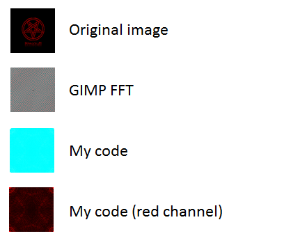
Great question. I’ve never heard of it but the Gimp Fourier plugin seems really neat:

A simple plug-in to do fourier transform on you image. The major advantage of this plugin is to be able to work with the transformed image inside GIMP. You can so draw or apply filters in fourier space, and get the modified image with an inverse FFT.

This idea—of doing Gimp-style manipulation on frequency-domain data and transforming back to an image—is very cool! Despite years of working with FFTs, I’ve never thought about doing this. Instead of messing with Gimp plugins and C executables and ugliness, let’s do this in Python!

Caveat. I experimented with a number of ways to do this, attempting to get something close to the output Gimp Fourier image (gray with moiré pattern) from the original input image, but I simply couldn’t. The Gimp image appears to be somewhat symmetric around the middle of the image, but it’s not flipped vertically or horizontally, nor is it transpose-symmetric. I’d expect the plugin to be using a real 2D FFT to transform an H×W image into a H×W array of real-valued data in the frequency domain, in which case there would be no symmetry (it’s just the to-complex FFT that’s conjugate-symmetric for real-valued inputs like images). So I gave up trying to reverse-engineer what the Gimp plugin is doing and looked at how I’d do this from scratch.

The code. Very simple: read an image, apply scipy.fftpack.rfft in the leading two dimensions to get the “frequency-image”, rescale to 0–255, and save.

Note how this is different from the other answers! No grayscaling—the 2D real-to-real FFT happens independently on all three channels. No abs needed: the frequency-domain image can legitimately have negative values, and if you make them positive, you can’t recover your original image. (Also a nice feature: no compromises on image size. The size of the array remains the same before and after the FFT, whether the width/height is even or odd.)

from PIL import Image
import numpy as np
import scipy.fftpack as fp

## Functions to go from image to frequency-image and back
im2freq = lambda data: fp.rfft(fp.rfft(data, axis=0),
                               axis=1)
freq2im = lambda f: fp.irfft(fp.irfft(f, axis=1),
                             axis=0)

## Read in data file and transform
data = np.array(Image.open('test.png'))

freq = im2freq(data)
back = freq2im(freq)
# Make sure the forward and backward transforms work!
assert(np.allclose(data, back))

## Helper functions to rescale a frequency-image to [0, 255] and save
remmax = lambda x: x/x.max()
remmin = lambda x: x - np.amin(x, axis=(0,1), keepdims=True)
touint8 = lambda x: (remmax(remmin(x))*(256-1e-4)).astype(int)

def arr2im(data, fname):
    out = Image.new('RGB', data.shape[1::-1])
    out.putdata(map(tuple, data.reshape(-1, 3)))
    out.save(fname)

arr2im(touint8(freq), 'freq.png')

(Aside: FFT-lover geek note. Look at the documentation for rfft for details, but I used Scipy’s FFTPACK module because its rfft interleaves real and imaginary components of a single pixel as two adjacent real values, guaranteeing that the output for any-sized 2D image (even vs odd, width vs height) will be preserved. This is in contrast to Numpy’s numpy.fft.rfft2 which, because it returns complex data of size width/2+1 by height/2+1, forces you to deal with one extra row/column and deal with deinterleaving complex-to-real yourself. Who needs that hassle for this application.)

Results. Given input named test.png:

this snippet produces the following output (global min/max have been rescaled and quantized to 0-255):

And upscaled:

In this frequency-image, the DC (0 Hz frequency) component is in the top-left, and frequencies move higher as you go right and down.

Now, let’s see what happens when you manipulate this image in a couple of ways. Instead of this test image, let’s use a cat photo.

I made a few mask images in Gimp that I then load into Python and multiply the frequency-image with to see what effect the mask has on the image.

Here’s the code:

# Make frequency-image of cat photo
freq = im2freq(np.array(Image.open('cat.jpg')))

# Load three frequency-domain masks (DSP "filters")
bpfMask = np.array(Image.open('cat-mask-bpfcorner.png')).astype(float) / 255
hpfMask = np.array(Image.open('cat-mask-hpfcorner.png')).astype(float) / 255
lpfMask = np.array(Image.open('cat-mask-corner.png')).astype(float) / 255

# Apply each filter and save the output
arr2im(touint8(freq2im(freq * bpfMask)), 'cat-bpf.png')
arr2im(touint8(freq2im(freq * hpfMask)), 'cat-hpf.png')
arr2im(touint8(freq2im(freq * lpfMask)), 'cat-lpf.png')

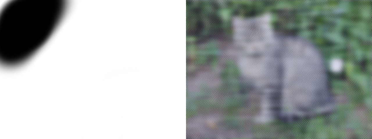
Here’s a low-pass filter mask on the left, and on the right, the result—click to see the full-res image:

In the mask, black = 0.0, white = 1.0. So the lowest frequencies are kept here (white), while the high ones are blocked (black). This blurs the image by attenuating high frequencies. Low-pass filters are used all over the place, including when decimating (“downsampling”) an image (though they will be shaped much more carefully than me drawing in Gimp 😜).

Here’s a band-pass filter, where the lowest frequencies (see that bit of white in the top-left corner?) and high frequencies are kept, but the middling-frequencies are blocked. Quite bizarre!

Here’s a high-pass filter, where the top-left corner that was left white in the above mask is blacked out:

This is how edge-detection works.

Postscript. Someone, make a webapp using this technique that lets you draw masks and apply them to an image real-time!!!

Brachy

Thank you for great explanation, but it seems that it's not exactly what I'm looking for. I used fft plugin from gimp on cat Image and its seems to look different. And I have a lot of problems with scipy library on my machine. – Thesaurus

Is your goal to exactly replicate the Gimp Fourier plugin's behavior? I can take a look at that source code and try to figure out what it’s doing—the examples you showed make no sense. Nonetheless, the approach in my code is very general, and examples show that it works well, so if you just need functionality similar to the plugin, the code works well. – Brachy

What system do you have that you’re having problems installing scipy? – Brachy

This website let you customize masks and apply them to an image. bigwww.epfl.ch/demo/ip/demos/03-FFT-filtering – Sequester

@CristianArteaga it's now over at bigwww.epfl.ch/demo/ip/demos/FFT-filtering - but very cool, thanks for sharing the link! – Toothed

I'm getting this error: [TypeError: argument must be a sequence] Anyone know about it? – Gondi

@Gondi which line? – Brachy

I thinik it is stopping here "out.putdata(map(tuple, data.reshape(-1, 3)))" because after this line in console it shows line 1566 in Image.py – Gondi

Answer 2

There are several issues here.

1) Manual conversion to grayscale isn't good. Use Image.open("test.png").convert('L')

2) Most likely there is an issue with types. You shouldn't pass np.ndarray from fft2 to a PIL image without being sure their types are compatible. abs(np.fft.fft2(something)) will return you an array of type np.float32 or something like this, whereas PIL image is going to receive something like an array of type np.uint8.

3) Scaling suggested in the comments looks wrong. You actually need your values to fit into 0..255 range.

Here's my code that addresses these 3 points:

import numpy as np
from PIL import Image

def fft(channel):
    fft = np.fft.fft2(channel)
    fft *= 255.0 / fft.max()  # proper scaling into 0..255 range
    return np.absolute(fft)

input_image = Image.open("test.png")
channels = input_image.split()  # splits an image into R, G, B channels
result_array = np.zeros_like(input_image)  # make sure data types, 
# sizes and numbers of channels of input and output numpy arrays are the save

if len(channels) > 1:  # grayscale images have only one channel
    for i, channel in enumerate(channels):
        result_array[..., i] = fft(channel)
else:
    result_array[...] = fft(channels[0])

result_image = Image.fromarray(result_array)
result_image.save('out.png')

I must admit I haven't managed to get results identical to the GIMP FFT plugin. As far as I see it does some post-processing. My results are all kinda very low contrast mess, and GIMP seems to overcome this by tuning contrast and scaling down non-informative channels (in your case all chanels except Red are just empty). Refer to the image:

Limeade