How to Bound the Outer Area of Voronoi Polygons and Intersect with Map Data

Question

Background

I'm trying to visualize the results of a kmeans clustering procedure on the following data using voronoi polygons on a US map.

Here is the code I've been running so far:

input <- read.csv("LatLong.csv", header = T, sep = ",")

# K Means Clustering

set.seed(123)
km <- kmeans(input, 17)
cent <- data.frame(km$centers)


# Visualization
states <- map_data("state")
StateMap <- ggplot() + geom_polygon(data = states, aes(x = long, y = lat, group = group), col = "white")

# Voronoi
V <- deldir(cent$long, cent$lat)

ll <-apply(V$dirsgs, 1, FUN = function(x){
  readWKT(sprintf("LINESTRING(%s %s, %s %s)", x[1], x[2], x[3], x[4]))
})

pp <- gPolygonize(ll)=
v_df <- fortify(pp)


# Plot
StateMap +
  geom_point(data = input, aes(x = long, y = lat), col = factor(km$cluster)) +
  geom_polygon(data = v_df, aes(x = long, y = lat, group = group, fill = id), alpha = .3) +
  geom_label(data = cent, aes(x = long, y = lat, label = row.names(cent)), alpha = .3)

Producing the Following

Question

I'd like to be able to bind the outer area of the polygons and intersect the resulting area with my map of the United States so that the polygons entirely represent US land area. I haven't been able to figure out how to do this though. Any help is greatly appreciated.

Weiser

Answer 1

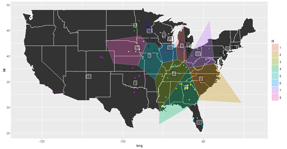
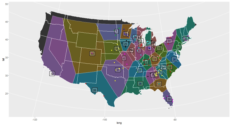
My end goal in asking this question was to write a script where I can arbitrarily change the number of kmeans clusters and quickly visualize the results with voronoi polygons that cover my desired area region.

I haven't quite accomplished this yet, but I have made enough progress that I figured posting what I have may lead to a quicker solution.

# Create Input Data.Frame
input <- as.data.frame(cbind(x$long, x$lat))
colnames(input) <- c("long", "lat")

# Set Seed and Run Clustering Procedure
set.seed(123)
km <- kmeans(input, 35)

# Format Output for Plotting
centers <- as.data.frame(cbind(km$centers[,1], km$centers[,2]))
colnames(centers) <- c("long", "lat")
cent.id <- cbind(ID = 1:dim(centers)[1], centers)

# Create Spatial Points Data Frame for Calculating Voronoi Polygons
coords  <- centers[,1:2]
vor_pts <- SpatialPointsDataFrame(coords, centers, proj4string = CRS("+proj=longlat +datum=WGS84"))

I also found the below.function while searching for a solution online.

# Function to Extract Voronoi Polygons 

SPdf_to_vpoly <- function(sp) {
  
  # tile.list extracts the polygon data from the deldir computation
  vor_desc <- tile.list(deldir(sp@coords[,1], sp@coords[,2]))
  
  lapply(1:length(vor_desc), function(i) {
    
    # tile.list gets us the points for the polygons but we 
    # still have to close them, hence the need for the rbind
    
    tmp <- cbind(vor_desc[[i]]$x, vor_desc[[i]]$y)
    tmp <- rbind(tmp, tmp[1,])
    
    # Now we can make the polygons
    Polygons(list(Polygon(tmp)), ID = i)
  }) -> vor_polygons
  # Hopefully the caller passed in good metadata
  sp_dat <- sp@data
  
  # This way the IDs should match up with the data & voronoi polys
  rownames(sp_dat) <- sapply(slot(SpatialPolygons(vor_polygons), 'polygons'), slot, 'ID')
  
  SpatialPolygonsDataFrame(SpatialPolygons(vor_polygons), data = sp_dat)
}

With the above function defined polygons can be extracted accordingly

vor     <- SPdf_to_vpoly(vor_pts)
vor_df  <- fortify(vor)

In order to get the voronoi polygons to fit nicely with a US map I downloaded cb_2014_us_state_20m from the Census website and ran the following:

# US Map Plot to Intersect with Voronoi Polygons - download from census link and place in working directory
us.shp <- readOGR(dsn = ".", layer = "cb_2014_us_state_20m")
state.abb <- state.abb[!state.abb %in% c("HI", "AK")]

Low48 <- us.shp[us.shp@data$STUSPS %in% state.abb,]

# Define Area Polygons and Projections and Calculate Intersection
Low48.poly <- as(Low48, "SpatialPolygons")
vor.poly   <- as(vor, "SpatialPolygons")

proj4string(vor.poly) <- proj4string(Low48.poly)
intersect  <- gIntersection(vor.poly, Low48.poly, byid = T)


# Convert to Data Frames to Plot with ggplot
Low48_df <- fortify(Low48.poly)
int_df   <- fortify(intersect)

From here I could visualize my results using ggplot like before:

# Plot Results
StateMap <- ggplot() + geom_polygon(data = Low48_df, aes(x = long, y = lat, group = group), col = "white")

StateMap +
  geom_polygon(data = int_df, aes(x = long, y = lat, group = group, fill = id), alpha = .4) +
  geom_point(data = input, aes(x = long, y = lat), col = factor(km$cluster)) +
  geom_label(data = centers, aes(x = long, y = lat, label = row.names(centers)), alpha =.2) +
  scale_fill_hue(guide = 'none') +
  coord_map("albers", lat0 = 30, lat1 = 40)

Summary of Updates

The overlapping voronoi polygons still aren't a perfect fit (I'm guessing due to a lack of input data in the pacific northwest) although I'd imagine that should be a simple fix and I'll try to update that as soon as possible. Also if I alter the number of kmeans centroids in the beginning of my function and then re-run everything the polygons don't look very nice at all which is not what I was originally hoping for. I'll continue to update with improvements.

Weiser