How to inner-join in Excel (eg. using VLOOKUP)

Question

Is there a way to inner join two different Excel spreadsheets using VLOOKUP?

In SQL, I would do it this way:

SELECT id, name
FROM Sheet1
INNER JOIN Sheet2
ON Sheet1.id = Sheet2.id;

Sheet1:

+----+------+
| ID | Name |
+----+------+
|  1 | A    |
|  2 | B    |
|  3 | C    |
|  4 | D    |
+----+------+

Sheet2:

+----+-----+
| ID | Age |
+----+-----+
|  1 |  20 |
|  2 |  21 |
|  4 |  22 |
+----+-----+

And the result would be:

+----+------+
| ID | Name |
+----+------+
|  1 | A    |
|  2 | B    |
|  4 | D    |
+----+------+

How can I do this in VLOOKUP? Or is there a better way to do this besides VLOOKUP?

Thanks.

Lacedaemonian

Did you try? =VLOOKUP(Sheet2!A1,Sheet1!A:B,2,False) Where column A:A in both sheets hold the id and Column B on Sheet 1 has the name. It would go in B1 in Sheet 2 and copied down. – Geodynamics

Is there a way for it to return the columns with the IDs as well? – Lacedaemonian

So you want to populate a new sheet with only the ids found in both sheets and the corresponding name from sheet 1? Will there ever be a time that there are ids on sheet 2 that are not on sheet 1? – Geodynamics

VLOOKUP won't duplicate rows. For example if two rows of 'A' in table1 matches three rows 'A' in table2, an inner join will result in six rows and VLOOKUP will result in two rows. If there are no matches VLOOKUP results in a row and inner join results in none – Casa

@ScottCraner Yes, and yes. In the latter's case, it would look like this. – Lacedaemonian

@Nick.McDermaid Is there another way to do Inner Join in Excel's formula bar? – Lacedaemonian

Could you mock up some data? – Geodynamics

@ScottCraner Done. I edited my post. – Lacedaemonian

You can use Microsoft Queries to make inner joins – Atalanta

how would the data be displayed if the id is in sheet2 but not in sheet1? Would it even be in the output? – Geodynamics

@Atalanta I can't use MS Queries because I'm doing this through Java's JDBC. – Lacedaemonian

@PuggyLongLegs doesn't matter because wou can make queries along worksheets themself – Atalanta

@ScottCraner The same thing will happen vice versa of my example. The result should only display rows that contain IDs that can be found in both sheets, since I'm inner-joining where the Sheet1's ID = Sheet2's ID. – Lacedaemonian

@Atalanta I can't because I'm going to be working with tables that are not in the same server. – Lacedaemonian

@PuggyLongLegs I know, if you are able to store your values in a worksheet, microsoft Query will work. The query will be executed on the sheets, not on the data object. let me post an answer. – Atalanta

Answer 1

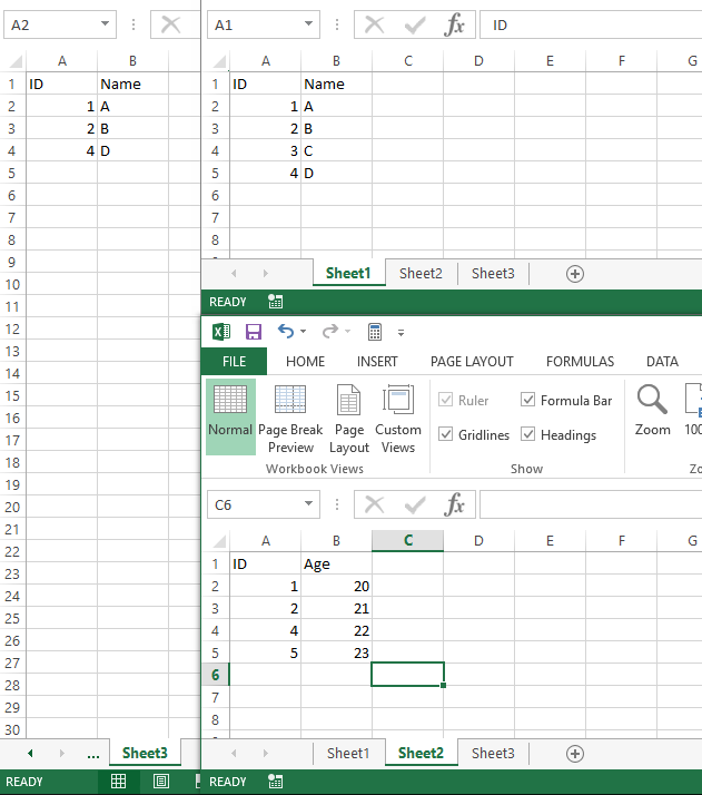
First lets get a list of values that exist in both tables. If you are using excel 2010 or later then in Sheet 3 A2 put the following formula:

=IFERROR(AGGREGATE(15,6,Sheet2!$A$1:$A$5000/(COUNTIF(Sheet1!$A$1:$A$5000,Sheet2!$A$1:$A$5000)>0),ROW(1:1)),"")

If you are using 2007 or earlier then use this array formula:

=IFERROR(SMALL(IF(COUNTIF(Sheet1!$A$1:$A$5000,Sheet2!$A$1:$A$5000),Sheet2!$A$1:$A$5000),ROW(1:1)),"")

Being an array formula, copy and paste into the formula bar then hit Ctrl-Shift-Enter instead of Enter or Tab to leave the edit mode.

Then copy down as many rows as desired. This will create a list of ID'd that are in both lists. This does assume that ID is a number and not text.

Then with that list we use vlookup:

=IF(A2<>"",VLOOKUP(A2,Sheet1!A:B,2,FALSE),"")

This will then return the value from Sheet 1 that matches.

Geodynamics

Thanks. What do you mean by copying rows? – Lacedaemonian

@PuggyLongLegs Drag the formula down as far as you want. As it drags it will copy the formulas down and change the references. – Geodynamics

I did this but when I pressed enter, nothing happened. I have the exact same Sheet1 and Sheet2. – Lacedaemonian

What excel are you using? @PuggyLongLegs – Geodynamics

@PuggyLongLegs see edit, the original formula was for 2010 or later, I have added a formula for 2007 or earlier. – Geodynamics

This actually worked. Now I just need to see if I can incorporate this in my program without problems. Thanks very much. – Lacedaemonian

@PuggyLongLegs please mark as correct, by clicking on the green check mark by the answer as it answers the question posed. – Geodynamics

Answer 2

You can acheive this result using Microsoft Query.

First, select Data > From other sources > From Microsoft Query

Then select "Excel Files*".

In the "Select Workbook" windows, you have to select the current Workbook.

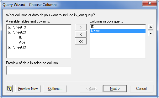
Next, in the query Wizard windows, select sheet1$ and sheet2$ and click the ">" button.

Click Next and the query visual editor will open.

Click on the SQL button and paste this query :

SELECT `Sheet1$`.ID, `Sheet1$`.Name, `Sheet2$`.Age
FROM`Sheet1$`, `Sheet2$`
WHERE `Sheet1$`.ID = `Sheet2$`.ID

Finally close the editor and put the table where you need it.

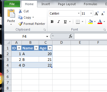
The result should look like this :

Atalanta

Thanks, but my problem is that I have to do all these through Java (using JDBC & Apache POI). The only thing Excel will do by itself is display the results of calculations and logic from my Java code. – Lacedaemonian

You can put this in your template Workbook and then call "update all" before displaying the result of the calculations – Atalanta

But my tables, columns, and conditions are dynamic. Unless I can create a template Workbook manually on Java every time I run my program. – Lacedaemonian

Answer 3

For Basic Excel Join without formuales or Excel Macros. Please check the website http://exceljoins.blogspot.com/2013/10/excel-inner-join.html

Joins can Left Outer, Right Outer and Full Outer which used in rare ocassions, But we can achieve this for Excel Sheets, For more information check the below http://exceljoins.blogspot.com/

Monophagous

For Basic Excel Join without formuales or Excel Macros. Please check the website exceljoins.blogspot.com/2013/10/excel-inner-join.html Joins can Left Outer, Right Outer and Full Outer which used in rare ocassions, But we can achieve this for Excel Sheets, For more information check the below exceljoins.blogspot.com – Monophagous

Please post the relevant sections of the answer here itself as links might change over time. – Susian