How can we perform common set operations (union, intersection, minus) in MS Excel?

Question

For example, I have an xls where :

• column A has list of items with property A
• column B has list of items with property B

I need the following :

• column C which is A union B (unique items of both A & B)
• column D which is A intersection B (common items of A & B)
• column E which is A minus B (items in A but not in B)
• column F which is B minus A (items in B but not in A)

Set operations on a list of elements seem to be easy with SQL or Python. But how to do it in xls?

Note : It should be an automation with minimal copy-pastes and clicks. For example, I dont want to copy-paste A below B, then "eliminate duplicates" to get A union B.

Outstay

Are you pulling this data from a database? If so it would be much easier to apply a union and/or intersection on the data their rather than in excel – Diagraph

No, the data was in csv files. – Outstay

Answer 1

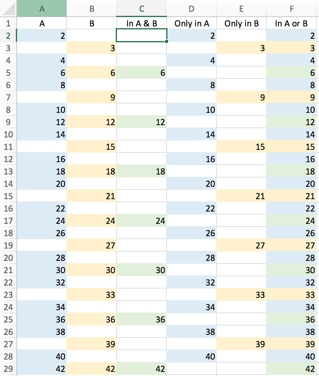
Intersection (In A & B): =IFNA(VLOOKUP(B2,$A$2:$B$42,1,FALSE),"")

Union (In A or B): =IFS(A2,A2,B2,B2) Note that IFS is only in Office 2019 and newer editions.

A - B (Only in A): =IF(NOT(IFNA(MATCH(A2,$B$2:$B$42,0),FALSE)),IF(A2,A2,""),"")

B - A (Only in B): =IF(NOT(IFNA(MATCH(B2,$A$2:$A$42,0),FALSE)),IF(B2,B2,""),"") (Swap the letters)

Ghost

Re. "IFS is only in recent (as of 2018) versions": a) not aware of an "Excel 2018" edition, closest edition would be "2016" or "2019", b) per MS docs (at "support.microsoft.com/en-us/office/…), Excel "IFS" function was introduced in "Excel 2019". – Odaodab

According to Wikipedia, Office 2019 was released on September 24, 2018 (US). You'll notice that this comment was written in December of 2018 as well. You are correct in surmising that, as of December 2018, the 'recent version' of Office was the 2019 edition. Perhaps next time you could suggest a help edit (I believe you should have sufficient reputation) rather than leaving an unhelpful pedantic comment. – Ghost

Answer 2

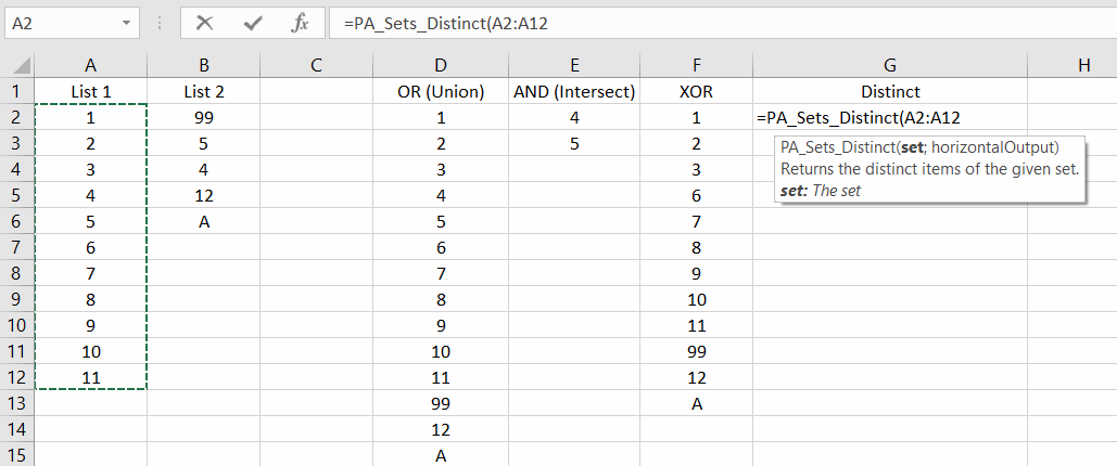
Excel alone seems not to be able to do the job. However, there are add-ins available. You might want to test the free and open source Power Analytics for Excel. It comes with some functions exactly performing what you asked for:

Usage in Excel 365

In Excel 365 Power Analytics for Excel allows to use dynamic arrays. This feature is exclusively included Excel 365 and not available in t Excel 2019, 2016 and so on.

In the following example we simply write =PA_Sets_And(A2:A11;B2:B6) into the single cell D2 and then - like magic - the formula expands to the required length of three rows.

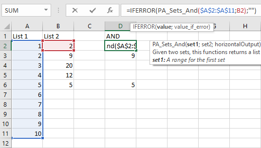
Usage in Excel 2019, 2016, ...

Here we use the PA_Sets_And method in order to look up whether the cell (B2) is contained in the range of the whole set (A2:A11). Not as cool as for Excel 365 but a little bit nicer than VLOOKUP :-)

Psalmist

Answer 3

Well, Microsoft Excel does not handle built-in set operations. But you can emulate then by VBA using MATCH function and error handling.

Here is the code that worked for me (I presume that you have heading on the first line):

Sub set_operations()
    Dim i, j, rangeA, rangeB, rowC, rowD, rowE, rowF As Long
    Dim test1, test2 As Boolean

    rangeA = ActiveSheet.Range("A" & CStr(ActiveSheet.Rows.Count)).End(xlUp).Row()
    rangeB = ActiveSheet.Range("B" & CStr(ActiveSheet.Rows.Count)).End(xlUp).Row()
    rowC = 2
    rowD = 2
    rowE = 2
    rowF = 2
    test1 = False
    test2 = False
    test2 = False

    'A union B
    On Error GoTo errHandler1
    For i = 2 To rangeA
        If Application.Match(ActiveSheet.Cells(i, 1), ActiveSheet.Range("C:C"), 0) > 0 Then
            If test1 = True Then
                ActiveSheet.Cells(rowC, 3) = ActiveSheet.Cells(i, 1)
                rowC = rowC + 1
            End If
        End If
        test1 = False
    Next i
    For j = 2 To rangeB
        If Application.Match(ActiveSheet.Cells(j, 2), ActiveSheet.Range("C:C"), 0) > 0 Then
            If test1 = True Then
                ActiveSheet.Cells(rowC, 3) = ActiveSheet.Cells(j, 2)
                rowC = rowC + 1
            End If
        End If
        test1 = False
    Next j

    'A intersection B
    For i = 2 To rangeA
        On Error GoTo errHandler2
        If Application.Match(ActiveSheet.Cells(i, 1), ActiveSheet.Range("B:B"), 0) > 0 Then
            On Error GoTo errHandler1
            If Application.Match(ActiveSheet.Cells(i, 1), ActiveSheet.Range("D:D"), 0) > 0 Then
                If test1 = True And test2 = False Then
                    ActiveSheet.Cells(rowD, 4) = ActiveSheet.Cells(i, 1)
                    rowD = rowD + 1
                End If
            End If
        End If
        test1 = False
        test2 = False
    Next i

    'A minus B
    For i = 2 To rangeA
        On Error GoTo errHandler2
        If Application.Match(ActiveSheet.Cells(i, 1), ActiveSheet.Range("B:B"), 0) > 0 Then
            On Error GoTo errHandler1
            If Application.Match(ActiveSheet.Cells(i, 1), ActiveSheet.Range("E:E"), 0) > 0 Then
                If test1 = True And test2 = True Then
                    ActiveSheet.Cells(rowE, 5) = ActiveSheet.Cells(i, 1)
                    rowE = rowE + 1
                End If
            End If
        End If
        test1 = False
        test2 = False
    Next i

    'B minus A
    For i = 2 To rangeB
        On Error GoTo errHandler2
        If Application.Match(ActiveSheet.Cells(i, 2), ActiveSheet.Range("A:A"), 0) > 0 Then
            On Error GoTo errHandler1
            If Application.Match(ActiveSheet.Cells(i, 2), ActiveSheet.Range("F:F"), 0) > 0 Then
                If test1 = True And test2 = True Then
                    ActiveSheet.Cells(rowF, 6) = ActiveSheet.Cells(i, 2)
                    rowF = rowF + 1
                End If
            End If
        End If
        test1 = False
        test2 = False
    Next i


errHandler1:
    test1 = True
    Resume Next

errHandler2:
    test2 = True
    Resume Next
End Sub

Spinks

its too much to do for simple operations like these.. Hoping there must be an easy way out. – Outstay

There are also private plugins for Excel which make what you want, like XLTools, but I never tested them. – Spinks

Perhaps this was the best option in 2015, but it is not as of today. – Ghost

Answer 4

you can simple use below formula to get result

=IF(LOWER(A4)=LOWER(B4),"",A4)

Hardened

Answer 5

I'm surprised at several levels:
(1) 2020 now .... and still no set functions in Excel
(2) The highest voted answer (from 2018) is very impractical: in real live, data sets don't come neatly with empty rows inserted where a value is missing vs. another data set; which is the precondition for this solution.

The most practical solution (though still awkward; do you hear us, Microsoft ???) is a work around with the help of a pivot table:

• Add column to set A, with column name "set_name" and all values in the column set to "A" -> pivot input A
• Add column to set B, with column name "set_name" and all values in the column set to "B" -> pivot input B
• copy pivot input B (without column names ;-)) under pivot input A to form a joint range -> joint range
• create a pivot table from the joint range with
  --- "set names" being used to form the columns of the pivot table
  --- pivot function set to "count()"

The result is a sort of "one-hot-encoded" pivot table with:

• 1st column: union set of A and B (aka ALL occuring values)
• 2nd column: 1-values only for elements occuring in set A
  (caveat: assumption is that A only contains UNIQUE elements. Otherwise,
  values > 1 are possible)
• 3rd column: 1-values only for elements occuring in set B
  (same caveat applies as for set A)
• Total column: values showing "2" value exist in both sets

The resulting pivot table can easily be filtered on the different sets and intersections via the values in columns 2 (aka "set A"),3 (aka "set B") and 4 (aka "Set A AND Set B").

Virendra

The blank lines in my example are merely for illustration purposes and are by no means required for the equations to function correctly. – Ghost

Answer 6

RE: Intersection of Two Sets

This solution is for Microsoft 365 and builds upon a method I explained in another post.

1. We find which array contains the most elements to not miss any of them.
2. We leverage the SCAN formula to find the common values between the two arrays using an XLOOKUP inside the formula's function parameter as the body of a LAMBDA.
3. We FILTER the result excluding any NA values for whenever no much was found for an element of the lookup array and the other array.

The only modification to the code of the aforementioned post is to wrap the LET's calculation inside a UNIQUE formula so that we get an actual Set, as shown below:

=LAMBDA(array_a, array_b,
    LET(
        scanResult, IF(
            COUNTA(array_a) > COUNTA(array_b),
            SCAN(
                "",
                array_a,
                LAMBDA(accumulator, current, XLOOKUP(current, array_b, array_b))
            ),
            SCAN(
                "",
                array_b,
                LAMBDA(accumulator, current, XLOOKUP(current, array_a, array_a))
            )
        ),
        UNIQUE(FILTER(scanResult, NOT(ISNA(scanResult))))
    )
)

Spiel

Answer 7

I have a complex formula that can do A-B set operation in Excel [checked in Microsoft365].:

=UNIQUE(
       LET(A_array,"A_Range",B_array,"B_Range",
             MAP(A_array,LAMBDA(A_value,
                       REDUCE(A_value,B_array,LAMBDA(x,B_value,IF(x=B_value,"",x)))
))))

two loops are needed for the operation. first "MAP" function works like a simple loop. Supplying elements of Array A [A_value]. The second loop along with check is accomplished by REDUCE. Inside REDUCE, starter value is set as "A_value" and its lambda uses same value for x.

Indigence