Showing equation of nls model with ggpmisc

Question

R package ggpmisc can be used to show equation of lm model and poly model on ggplot2 (See here for reference). I wonder how I could show nls model equation results on ggplot2 using ggpmisc. Below is my MWE.

library(ggpmisc)
args <- list(formula = y ~ k * e ^ x,
             start = list(k = 1, e = 2))
ggplot(mtcars, aes(wt, mpg)) +
  geom_point() +
  stat_fit_augment(method = "nls",
                   method.args = args)

Britisher

Answer 1

It is also possible to add the equation using package 'ggpmisc', assembling the character string to be parsed with paste() or sprintf(). In this answer I will use sprintf(). I answer the question using the example it included. I do not show this in this answer, but this approach supports grouping and facets. The drawback is that the model is fit twice, once to draw the fitted line and once to add the equation.

To find the names of the variables returned by stat_fit_tidy() I used geom_debug() from package 'gginnards', although the names even if dependent on the model formula and method are rather easy to predict. Instead of adding a plot layer geom_debug() echoes is data input to the R console. Next, once we know the names of the variables we wish to use in the label, we can assemble the string to be parsed as an R expression.

When assembling the label with sprintf() one needs to escape the % characters to be returned unchanged as %%, so the multiplication sign %*% becomes %%*%%. It is possible, and in this case useful to embed character strings in the R expression, but we need to escape the embedded quotation marks as \".

library(tidyverse)
library(ggpmisc)
#> Loading required package: ggpp
#> 
#> Attaching package: 'ggpp'
#> The following object is masked from 'package:ggplot2':
#> 
#>     annotate
library(gginnards)

args <- list(formula = y ~ k * e ^ x,
             start = list(k = 1, e = 2))

# we find the names of computed values
ggplot(mtcars, aes(wt, mpg)) +
  stat_fit_tidy(method = "nls",
                method.args = args,
                geom = "debug")

#> Input 'data' to 'draw_panel()':
#>   npcx npcy k_estimate e_estimate     k_se       e_se   k_stat   e_stat
#> 1   NA   NA   49.65969  0.7455911 3.788755 0.01985924 13.10713 37.54378
#>      k_p.value    e_p.value       x      y fm.class fm.method  fm.formula
#> 1 5.963165e-14 8.861929e-27 1.70855 32.725      nls       nls y ~ k * e^x
#>   fm.formula.chr PANEL group
#> 1    y ~ k * e^x     1    -1

# plot with formula
ggplot(mtcars, aes(wt, mpg)) +
  geom_point() +
  stat_fit_augment(method = "nls",
                   method.args = args) +
  stat_fit_tidy(method = "nls",
                method.args = args,
                label.x = "right",
                label.y = "top",
                aes(label = sprintf("\"mpg\"~`=`~%.3g %%*%% %.3g^{\"wt\"}",
                                    after_stat(k_estimate),
                                    after_stat(e_estimate))),
                parse = TRUE )

^{Created on 2022-09-02 with reprex v2.0.2}

Toowoomba

Error in check_subclass(): ! Can't find geom called 'debug' – Almeria

Did you run library(gginnards)? – Toowoomba

Answer 2

Inspired by the post you linked. Use geom_text to add the label after extracting parameters.

nlsFit <-
  nls(formula = mpg ~ k * e ^ wt,
      start = list(k = 1, e = 2),
      data = mtcars)

nlsParams <-
  nlsFit$m$getAllPars()

nlsEqn <-
  substitute(italic(y) == k %.% e ^ italic(x), 
             list(k = format(nlsParams['k'], digits = 4), 
                  e = format(nlsParams['e'], digits = 2)))

nlsTxt <-
  as.character(as.expression(nlsEqn))

ggplot(mtcars, aes(wt, mpg)) +
  geom_point() +
  stat_fit_augment(method = "nls",
                   method.args = args) + 
  geom_text(x = 5, y = 30, label = nlsTxt, parse = TRUE)

Weinshienk

For some reason, the values ware encapsulated by c(). y = c(value) e ^ c(value): nlsTxt [1] "italic(y) == c(k = \"49.66\") %.% c(e = \"0.75\")^italic(x)" – Almeria

Answer 3

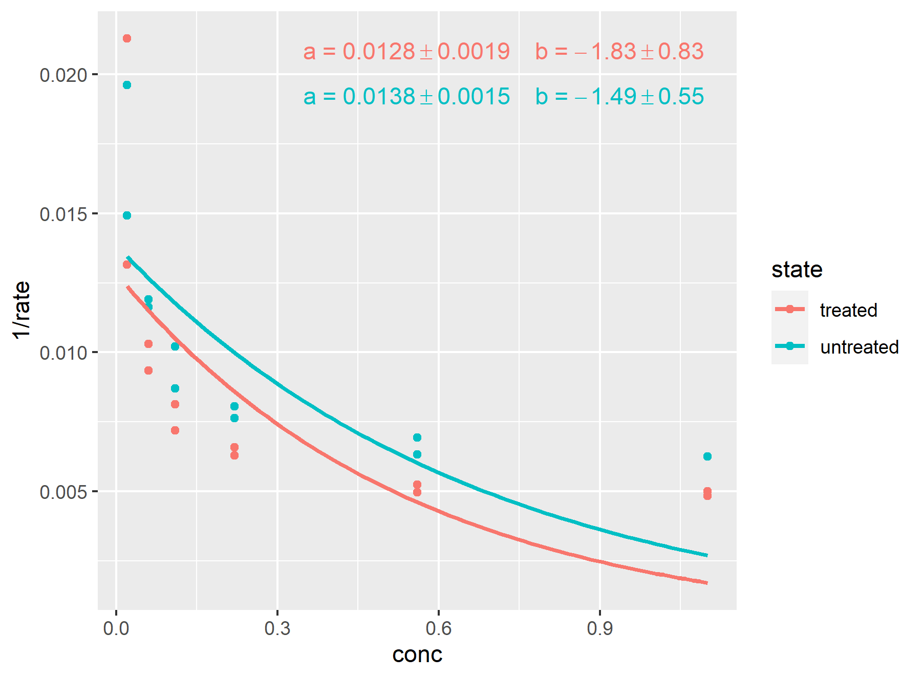
Here I have shown nls with groups using ggpmisc to add to the plots, using the current CRAN ggpmisc (v 0.3.8). This is a variation/modification of the vignette where 'stat_fit_tidy()' used a michaelis-menten fit, found here. Output looks like this:

library(tidyverse)
library(tidymodels)
library(ggpmisc)

my_exp_formula <-  y ~ a * exp(b*x-0)
# if x has large values (i.e. >700), subtract the minimum
# see https://mcmap.net/q/751364/-exponential-fit-in-ggplot-r

#example with nls, shows the data returned
o <- nls(1/rate ~ a * exp(b*conc-0), data = Puromycin, start = list(a = 1, b = 2))
o
tidy(o)

ggplot(Puromycin, aes(conc, 1/rate, colour = state)) +
  geom_point() +
  geom_smooth(method = "nls", 
              formula = my_exp_formula,
              se = FALSE) +
  stat_fit_tidy(method = "nls", 
                method.args = list(formula = my_exp_formula),
                label.x = "right",
                label.y = "top",
                aes(label = paste("a~`=`~", signif(stat(a_estimate), digits = 3),
                                  "%+-%", signif(stat(a_se), digits = 2),
                                  "~~~~b~`=`~", signif(stat(b_estimate), digits = 3),
                                  "%+-%", signif(stat(b_se), digits = 2),
                                  sep = "")),
                parse = TRUE)
ggsave("exp plot.png")

Benson