PyTorch Binary Classification - same network structure, 'simpler' data, but worse performance?

Question

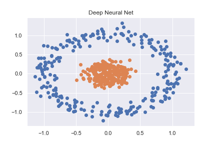
To get to grips with PyTorch (and deep learning in general) I started by working through some basic classification examples. One such example was classifying a non-linear dataset created using sklearn (full code available as notebook here)

n_pts = 500
X, y = datasets.make_circles(n_samples=n_pts, random_state=123, noise=0.1, factor=0.2)
x_data = torch.FloatTensor(X)
y_data = torch.FloatTensor(y.reshape(500, 1))

This is then accurately classified using a pretty basic neural net

class Model(nn.Module):
    def __init__(self, input_size, H1, output_size):
        super().__init__()
        self.linear = nn.Linear(input_size, H1)
        self.linear2 = nn.Linear(H1, output_size)

    def forward(self, x):
        x = torch.sigmoid(self.linear(x))
        x = torch.sigmoid(self.linear2(x))
        return x

    def predict(self, x):
        pred = self.forward(x)
        if pred >= 0.5:
            return 1
        else:
            return 0

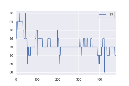
As I have an interest in health data I then decided to try and use the same network structure to classify some a basic real-world dataset. I took heart rate data for one patient from here, and altered it so all values > 91 would be labelled as anomalies (e.g. a 1 and everything <= 91 labelled a 0). This is completely arbitrary, but I just wanted to see how the classification would work. The complete notebook for this example is here.

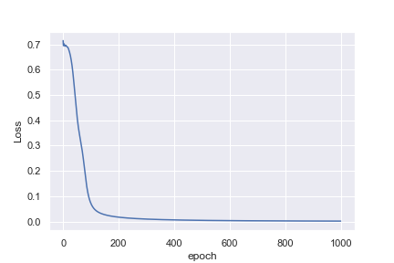
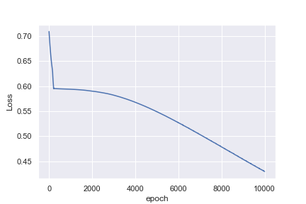
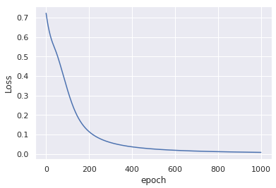
What is not intuitive to me is why the first example reaches a loss of 0.0016 after 1,000 epochs, whereas the second example only reaches a loss of 0.4296 after 10,000 epochs

Perhaps I am being naive in thinking that the heart rate example would be much easier to classify. Any insights to help me understand why this is not what I am seeing would be great!

Tourane

thank you very much for the bounty. Glad I could help. – Priory

Answer 1

TL;DR

Your input data is not normalized.

1. use x_data = (x_data - x_data.mean()) / x_data.std()
2. increase the learning rate optimizer = torch.optim.Adam(model.parameters(), lr=0.01)

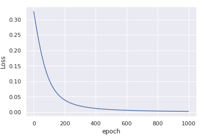
You'll get

convergence in only 1000 iterations.

More details

The key difference between the two examples you have is that the data x in the first example is centered around (0, 0) and has very low variance.
On the other hand, the data in the second example is centered around 92 and has relatively large variance.

This initial bias in the data is not taken into account when you randomly initialize the weights which is done based on the assumption that the inputs are roughly normally distributed around zero.
It is almost impossible for the optimization process to compensate for this gross deviation - thus the model gets stuck in a sub-optimal solution.

Once you normalize the inputs, by subtracting the mean and dividing by the std, the optimization process becomes stable again and rapidly converges to a good solution.

For more details about input normalization and weights initialization, you can read section 2.2 in He et al Delving Deep into Rectifiers: Surpassing Human-Level Performance on ImageNet Classification (ICCV 2015).

What if I cannot normalize the data?

If, for some reason, you cannot compute mean and std data in advance, you can still use nn.BatchNorm1d to estimate and normalize the data as part of the training process. For example

class Model(nn.Module):
    def __init__(self, input_size, H1, output_size):
        super().__init__()
        self.bn = nn.BatchNorm1d(input_size)  # adding batchnorm
        self.linear = nn.Linear(input_size, H1)
        self.linear2 = nn.Linear(H1, output_size)
    
    def forward(self, x):
        x = torch.sigmoid(self.linear(self.bn(x)))  # batchnorm the input x
        x = torch.sigmoid(self.linear2(x))
        return x

This modification without any change to the input data, yields similar convergance after only 1000 epochs:

A minor comment

For numerical stability, it is better to use nn.BCEWithLogitsLoss instead of nn.BCELoss. For this end, you need to remove the torch.sigmoid from the forward() output, the sigmoid will be computed inside the loss.
See, for example, this thread regarding the related sigmoid + cross entropy loss for binary predictions.

Priory

Quick follow-up question. How do I handle making predictions on new data, i.e. doesn't that also need to be normalized? But how can I do that if I just have a single new data point e.g. before you corrected my approach I would have simply used point = torch.tensor([100.]) and model.predict(point) – Marocain

@PhilipO'Brien you already have mean and STD computed once. You use these values throughout training and validation – Priory

@PhilipO'Brien see how it's done in the colab of the rnn answer I posted – Priory

So am I right in thinking you make the prediction with the new raw input data, and then multiple by the standard deviation and add the mean e.g. *sig+mu e.g. if point = torch.tensor([100.]) then pred = model.predict(point)*sig+mu – Marocain

I don't think I follow; in the colab you seem to apply mean and sig after generating the prediction e.e. pred[-1, ...]*sig + mu – Marocain

@PhilipO'Brien it goes both ways: you need to normalize the input and then "un normalize" the prediction: out=model((point-mu)/sig)*sig + mu – Priory

Ah sorry now I get you, I don't normalize the training data and the new input data. I normalize for training, and then predict using raw data, but "un normalize" the result of that prediction. Thanks again! – Marocain

@PhilipO'Brien wait a minute. In this task of predicting binary label you do not "un normalize" the output - it I binary and should remain so. In the other task of regressing continuous variables, there you have an issue of "un normalizing" the outputs – Priory

Answer 2

Let's start first by understanding how neural networks work, neural networks observe patterns, hence the necessity for large datasets. In the case of the example, two what pattern you intend to find is when if HR < 91: label = 0, this if-condition can be represented by the formula, sigmoid((HR-91) * 1) , if you plug various values into the formula you can see you that all values < 91, label 0 and others label 1. I have inferred this formula and it could be anything as long as it gives the correct values.

Basically, we apply the formula wx+b, where x in our input data and we learn the values for w and b. Now initially the values are all random, so getting the b value from 1030131190 (a random value), to maybe 98 is fast, since the loss is great, the learning rate allows the values to jump fast. But once you reach 98, your loss is decreasing, and when you apply the learning rate, it takes it more time to reach closer to 91, hence the slow decrease in loss. As the values get closer, the steps taken are even slower.

This can be confirmed via the loss values, they are constantly decreasing, initially, the deceleration is higher, but then it becomes smaller. Your network is still learning but slowly.

Hence in deep learning, you use this method called stepped learning rate, wherewith the increase in epochs you decrease your learning rate so that your learning is faster

Imminence

Thanks, I understand that process, but what I'm trying to understand is why it takes so much longer to achieve a low loss value for the second dataset. Both datasets are of a similar size, but the HR example would seem a more straightforward classification problem, but the training loss comparison suggests the opposite. – Marocain

This doesn't seem to try to answer OP's question. – Barnebas