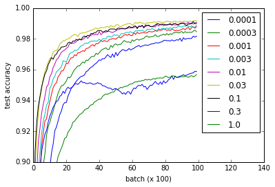
Regarding the MNIST tutorial on the TensorFlow website, I ran an experiment (gist) to see what the effect of different weight initializations would be on learning. I noticed that, against what I read in the popular [Xavier, Glorot 2010] paper, learning is just fine regardless of weight initialization.
The different curves represent different values for w for initializing the weights of the convolutional and fully connected layers. Note that all values for w work fine, even though 0.3 and 1.0 end up at lower performance and some values train faster - in particular, 0.03 and 0.1 are fastest. Nevertheless, the plot shows a rather large range of w which works, suggesting 'robustness' w.r.t. weight initialization.
def weight_variable(shape, w=0.1):
  initial = tf.truncated_normal(shape, stddev=w)
  return tf.Variable(initial)

def bias_variable(shape, w=0.1):
  initial = tf.constant(w, shape=shape)
  return tf.Variable(initial)
Question: Why does this network not suffer from the vanishing or exploding gradient problem?
I would suggest you read the gist for implementation details, but here's the code for reference. It took approximately an hour on my Nvidia 960m, although I imagine it could also run on a CPU within reasonable time.
import time
from tensorflow.examples.tutorials.mnist import input_data
import tensorflow as tf
from tensorflow.python.client import device_lib

import numpy
import matplotlib.pyplot as pyplot

mnist = input_data.read_data_sets('MNIST_data', one_hot=True)

# Weight initialization

def weight_variable(shape, w=0.1):
  initial = tf.truncated_normal(shape, stddev=w)
  return tf.Variable(initial)

def bias_variable(shape, w=0.1):
  initial = tf.constant(w, shape=shape)
  return tf.Variable(initial)


# Network architecture

def conv2d(x, W):
  return tf.nn.conv2d(x, W, strides=[1, 1, 1, 1], padding='SAME')

def max_pool_2x2(x):
  return tf.nn.max_pool(x, ksize=[1, 2, 2, 1],
                    strides=[1, 2, 2, 1], padding='SAME')

def build_network_for_weight_initialization(w):
    """ Builds a CNN for the MNIST-problem:
     - 32 5x5 kernels convolutional layer with bias and ReLU activations
     - 2x2 maxpooling
     - 64 5x5 kernels convolutional layer with bias and ReLU activations
     - 2x2 maxpooling
     - Fully connected layer with 1024 nodes + bias and ReLU activations
     - dropout
     - Fully connected softmax layer for classification (of 10 classes)

     Returns the x, and y placeholders for the train data, the output
     of the network and the dropbout placeholder as a tuple of 4 elements.
    """
    x = tf.placeholder(tf.float32, shape=[None, 784])
    y_ = tf.placeholder(tf.float32, shape=[None, 10])

    x_image = tf.reshape(x, [-1,28,28,1])
    W_conv1 = weight_variable([5, 5, 1, 32], w)
    b_conv1 = bias_variable([32], w)

    h_conv1 = tf.nn.relu(conv2d(x_image, W_conv1) + b_conv1)
    h_pool1 = max_pool_2x2(h_conv1)
    W_conv2 = weight_variable([5, 5, 32, 64], w)
    b_conv2 = bias_variable([64], w)

    h_conv2 = tf.nn.relu(conv2d(h_pool1, W_conv2) + b_conv2)
    h_pool2 = max_pool_2x2(h_conv2)

    W_fc1 = weight_variable([7 * 7 * 64, 1024], w)
    b_fc1 = bias_variable([1024], w)

    h_pool2_flat = tf.reshape(h_pool2, [-1, 7*7*64])
    h_fc1 = tf.nn.relu(tf.matmul(h_pool2_flat, W_fc1) + b_fc1)

    keep_prob = tf.placeholder(tf.float32)
    h_fc1_drop = tf.nn.dropout(h_fc1, keep_prob)

    W_fc2 = weight_variable([1024, 10], w)
    b_fc2 = bias_variable([10], w)

    y_conv = tf.matmul(h_fc1_drop, W_fc2) + b_fc2

    return (x, y_, y_conv, keep_prob)


# Experiment

def evaluate_for_weight_init(w):
    """ Returns an accuracy learning curve for a network trained on
    10000 batches of 50 samples. The learning curve has one item
    every 100 batches."""
    with tf.Session() as sess:
        x, y_, y_conv, keep_prob = build_network_for_weight_initialization(w)
        cross_entropy = tf.reduce_mean(
            tf.nn.softmax_cross_entropy_with_logits(labels=y_, logits=y_conv))
        train_step = tf.train.AdamOptimizer(1e-4).minimize(cross_entropy)
        correct_prediction = tf.equal(tf.argmax(y_conv,1), tf.argmax(y_,1))
        accuracy = tf.reduce_mean(tf.cast(correct_prediction, tf.float32))
        sess.run(tf.global_variables_initializer())
        lr = []
        for _ in range(100):
            for i in range(100):
                batch = mnist.train.next_batch(50)
                train_step.run(feed_dict={x: batch[0], y_: batch[1], keep_prob: 0.5})
            assert mnist.test.images.shape[0] == 10000
            # This way the accuracy-evaluation fits in my 2GB laptop GPU.
            a = sum(
                accuracy.eval(feed_dict={
                    x: mnist.test.images[2000*i:2000*(i+1)],
                    y_: mnist.test.labels[2000*i:2000*(i+1)],
                    keep_prob: 1.0})
                for i in range(5)) / 5
            lr.append(a)
        return lr


ws = [0.0001, 0.0003, 0.001, 0.003, 0.01, 0.03, 0.1, 0.3, 1.0]
accuracies = [
    [evaluate_for_weight_init(w) for w in ws]
    for _ in range(3)
]


# Plotting results

pyplot.plot(numpy.array(accuracies).mean(0).T)
pyplot.ylim(0.9, 1)
pyplot.xlim(0,140)
pyplot.xlabel('batch (x 100)')
pyplot.ylabel('test accuracy')
pyplot.legend(ws)


def evaluate_for_weight_init(w)andfor i in range(100):would you check it out – Pelag