Fitting a smooth spline (GAM function) in R: Error in number of knots required to fit spline -- knot requirements increasing

I'm trying to fit a smooth spline to what looks like data with two peaks. First, I fit a smooth spline to my data to identify the potential position of the knots.

library(npreg)
library(splines)
library(mgcv)

x <- c(20.70, 20.44, 20.58, 21.02, 19.90,  6.20,  8.20,  6.92,  5.86,  6.44,  6.34,  8.48,  8.46,  9.00,  9.06,  9.00,  9.06, 17.98, 18.42, 19.18, 22.88, 24.16,20.20, 23.50)

y <- c(19.884208, 12.772114, 12.932944,  5.016790, 11.405843,  3.310724,  3.950049,  3.641571,  4.073783,  4.616096,  3.425635,  7.773548,  7.498084, 9.474213,  6.162779, 11.041210, 12.618555,  6.287967,  4.286919,  3.242361,  7.571644,  3.379709,  5.274434,  8.8258)


data = data.frame(x,y)

fit_spline <- smooth.spline(x,y)
plot(x,y)
lines(fit_spline,lwd=2,col="purple")

Then, I wanted to run a regression using the gam function where I can specify the position of the knots. I get an error that says Error in smooth.construct.bs.smooth.spec(object, dk$data, dk$knots) : there should be 7 supplied knots I am not sure where it's drawing this number. If I supply 7 knots, it says it needs 13 knots...and the same erorr gets repeated. I am unclear on how to proceed.

myfit <- gam(y ~ s(x, bs = 'bs', k = 3),
             knots = list(x = c(1,5,20)))

my_knots <- myfit$smooth[[1]]$xp
plot(x, y, col= "grey", main = "my knots");
lines(x, myfit$linear.predictors, col = 2, lwd = 2)
abline(v = my_knots, lty = 2)

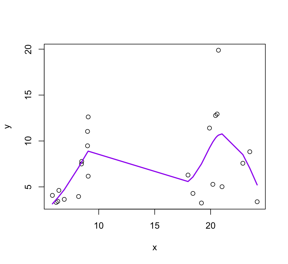
It looks like you came from one of my previous answer in 2016: mgcv: How to set number and / or locations of knots for splines, borrowing my code snippet:

my_knots <- myfit$smooth[[1]]$xp
plot(x, y, col= "grey", main = "my knots");
lines(x, myfit$linear.predictors, col = 2, lwd = 2)
abline(v = my_knots, lty = 2)

In that answer, my demonstration was made with cubic regression spline (bs = 'cr'), where knot placement is simple to do. But for B-splines, things are more complicated. So take this answer as a complement to that answer.

For B-spline classes in mgcv, i.e., 'bs' being "bs" (?b.spline), "ps" (?p.spline) or "ad" (?adaptive.smooth), the argument k is the number of B-splines, not the number of knots. And the first take-home message is: the number of B-splines is NOT equal to the number of knots.

Knot placement for B-splines is a dirty work. Usually you only specify k and mgcv will place knots automatically for you (see for example, Extract knots, basis, coefficients and predictions for P-splines in adaptive smooth). If you want to control knot placement yourself, the number of knots you provide must be compatible with k. This can cause great confusion if you don't well understand B-splines.

I highly recommend your reading the Appendix (page 33-34) of one of my work: General P-splines for Non-uniform B-splines, to know some fundamental stuff of B-splines. Make sure you understand what are the domain, interior knots and auxiliary boundary knots. In the following, I will just show you how to use these knowledge to write the correct code.

Here is how to place knots for your example.

## degree of spline
deg <- 3

## domain
a <- min(x)
#[1] 5.86
b <- max(x)
#[1] 24.16

## interior knots (must be between a and b)
xs <- c(6, 20)
#[1]  6 20

## domain knots
xd <- c(a, xs, b)
#[1]  5.86  6.00 20.00 24.16

## clamped auxiliary boundary knots
left.aux <- rep(a, deg)
#[1] 5.86 5.86 5.86
right.aux <- rep(b, deg)
#[1] 24.16 24.16 24.16

## complete B-spline knots
my.knots <- c(left.aux, xd, right.aux)
#[1]  5.86  5.86  5.86  5.86  6.00 20.00 24.16 24.16 24.16 24.16

Here is how to specify k for your example.

my.k <- length(xs) + deg + 1
#[1] 6

Now we can work with mgcv.

myfit <- gam(y ~ s(x, bs = 'bs', k = my.k),
             knots = list(x = my.knots))
#Family: gaussian 
#Link function: identity
#
#Formula:
#y ~ s(x, bs = "bs", k = my.k, m = deg)
#
#Estimated degrees of freedom:
#3.81  total = 4.81

The knots you passed in are stored here (which agree with my.knots):

## For B-spline classes, knots are stored in $knots instead of $xp
myfit$smooth[[1]]$knots
#[1]  5.86  5.86  5.86  5.86  6.00 20.00 24.16 24.16 24.16 24.16

Accompanying General P-splines for Non-uniform B-splines are R packages gps and gps.mgcv. The latter package introduces a new "gps" class to mgcv, where bs = 'ps' and bs = 'bs' are special cases of bs = 'gps'. The new "gps" class makes knot placement easier, because it automatically places auxiliary boundary knots for you and you only need to provide interior knots.

## The package stays on GitHub for the moment
## but will be on CRAN in the future.
## You may need to first install package 'devtools' from CRAN.
devtools::install_github("ZheyuanLi/gps")
devtools::install_github("ZheyuanLi/gps.mgcv")

library(gps.mgcv)

## as same as using 'bs = 'bs''
myfit <- gam(y ~ s(x, bs = 'gps', k = my.k, xt = list(derivative = TRUE)),
             knots = list(x = xs))  ## provide interior knots

## the novel general P-spline
gpsfit <- gam(y ~ s(x, bs = 'gps', k = my.k),
             knots = list(x = xs))  ## provide interior knots

Construction information (domain, interior knots, etc) are stored in myfit$smooth[[1]]$xt and gpsfit$smooth[[1]]$xt.

Recommended topics

Hot tags