Robust registration of two point clouds

Question

I need to find the transformation and rotation difference between two 3D point clouds. For this I am looking at Point Cloud Library, as it seems ideal.

On clean test data I have Iterative Closest Point (ICP) working, but getting strange results (although I may have implemented it incorrectly). I have pcl::estimateRigidTransformation working, and it seems better, although I assume will deal worse with noisy data.

My questions are:

The two clouds will be noisy, and although they should contain the same points, there will be some discrepancies. What is the best way to deal with this?

Should I find corresponding features in the two clouds to begin with and THEN use estimateTransform? Or should I look at a RANSAC function to remove outliers? Is ICP a better way to go than estimateRigidTransform?

Superfecundation

I'm new to PCL, so please pardon me if this is not useful. There's the PCL Registration library which I think will be useful for your purpose. – Wheaten

Just follow first some tutorials about ICP. And it depence on application Which filter you use, I really like the fast Voxel grid filter. ICP is not the best way to do so. First learn the examples and than build your own (from the trunk) pcl ICP. The ICP from the example is just a working function, instead you want a real preformer (a preformer ICP is an ICP that is build for you application) build your own! – Zoo

Answer 1

Setting up a robust point cloud registration algorithm can be a challenging task with a variaty of different options, hyperparameters and techniques to be set correctly to obtain strong results.

However the Point Cloud Library comes with a whole set of preimplemented function to solve this kind of task. The only thing left to do is to understand what each blocks is doing and to then set up a so called ICP Pipeline consisting of these blocks stacked on each other.

An ICP pipeline can follow two different paths:

1. Iterative registration algorithm

The easier path starts right away applying an Iterative Closest Point Algorithm on the Input-Cloud (IC) to math it with the fixed Reference-Cloud (RC) by always using the closest point method. The ICP takes an optimistic asumption that the two point clouds are close enough (good prior of rotation R and translation T) and the registration will converge without further initial alignment.

This path of course can get stucked in a local minimum and therefore perform very poorly as it is prone to get fooled by any kind of inaccuracies in the given input data.

2. Feature-based registration algorithm

To overcome this people have worked on developing all kinds of methods and ideas to overcome bad performing registration. In contrast to a merely iterative registration algorithm a feature-based registration first tires to find higher lever correspondences between the two point clouds to speed up the process and to improve the accuracy. The methods are capsuled and then embedded in the registration pipleline to form a complete registration model.

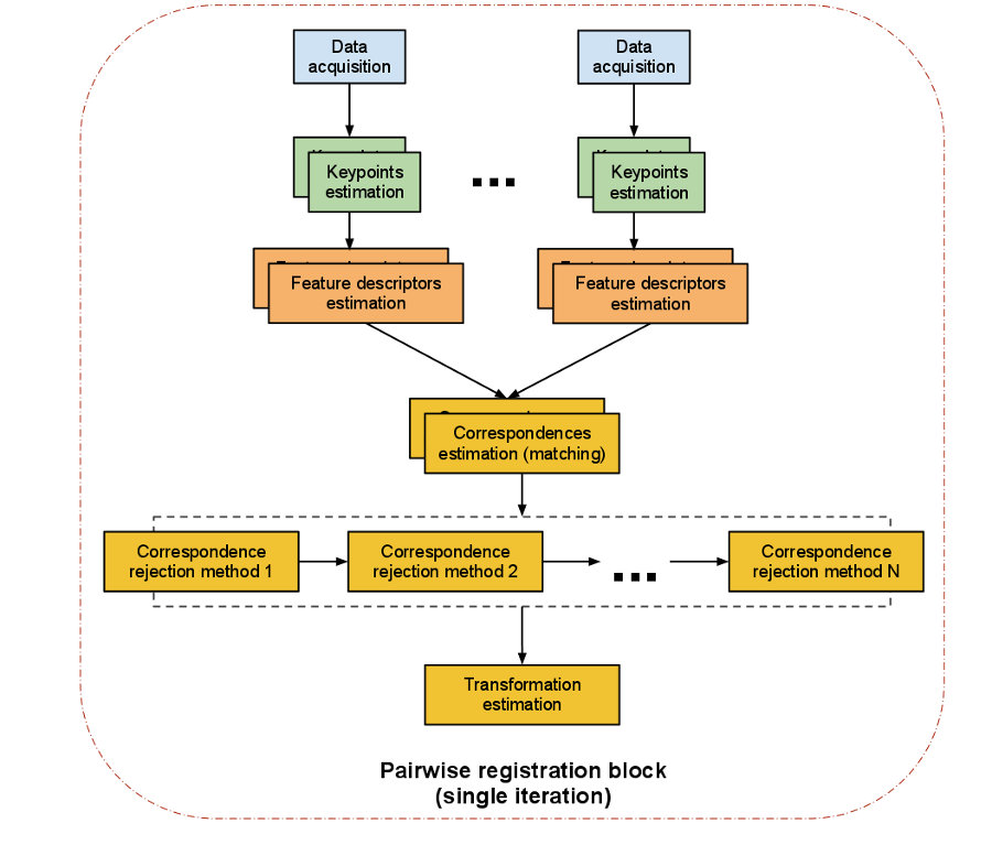
The following picture from the PCL documentation shows such a Registation pipeline:

As you can see a pairwise registration should run trough different computational steps to perform best. The single steps are:

1. Data acquisition: An input cloud and a reference cloud are fed into the algorithm.

2. Estimating Keypoints: A keypoint (interest point) is a point within the point cloud that has the following characteristics:

   1. it has a clear, preferably mathematically well-founded, definition,
   2. it has a well-defined position in image space,
   3. the local image structure around the interest point is rich in terms of local information contents

   Such salient points in a point cloud are so usefull because the sum of them characterizes a point cloud and helps making different parts of it distinguishable.

   pcl::NarfKeypoint
   pcl::ISSKeypoint3D< PointInT, PointOutT, NormalT >
   pcl::HarrisKeypoint3D< PointInT, PointOutT, NormalT >
   pcl::HarrisKeypoint6D< PointInT, PointOutT, NormalT >
   pcl::SIFTKeypoint< PointInT, PointOutT >
   pcl::SUSANKeypoint< PointInT, PointOutT, NormalT, IntensityT >
   

   Detailed Information: PCL Keypoint - Documentation

3. Describing keypoints - Feature descriptors: After detecting keypoints we go on to compute a descriptor for every one of them. "A local descriptor a compact representation of a point’s local neighborhood. In contrast to global descriptors describing a complete object or point cloud, local descriptors try to resemble shape and appearance only in a local neighborhood around a point and thus are very suitable for representing it in terms of matching." (Dirk Holz et al.)

   pcl::FPFHEstimation< PointInT, PointNT, PointOutT >
   pcl::NormalEstimation< PointInT, PointOutT >
   pcl::NormalEstimationOMP< PointInT, PointOutT >
   pcl::OURCVFHEstimation< PointInT, PointNT, PointOutT >
   pcl::PrincipalCurvaturesEstimation< PointInT, PointNT, PointOutT >
   pcl::IntensitySpinEstimation< PointInT, PointOutT >
   

   Detailed information: PCL Features - Documentation

4. Correspondence Estimation: The next task is to find correspondences between the keypoints found in the point clouds. Usually one takes advantage of the computed local featur-descriptors and match each one of them to his corresponding counterpart in the other point cloud. However due to the fact that two scans from a similar scene don't necessarily have the same number of feature-descriptors as one cloud can have more data then the other, we need to run a seperated correspondence rejection process.

   pcl::registration::CorrespondenceEstimation< PointSource, PointTarget, Scalar >
   pcl::registration::CorrespondenceEstimationBackProjection< PointSource, PointTarget, NormalT, Scalar >
   pcl::registration::CorrespondenceEstimationNormalShooting< PointSource, PointTarget, NormalT, Scalar >
   

5. Correspondence rejection: One of the most common approaches to perform correspondence rejection is to use RANSAC (Random Sample Consensus). But PCL comes with more rejection algorithms that a worth it giving them a closer look:

   pcl::registration::CorrespondenceRejectorSampleConsensus< PointT >
   pcl::registration::CorrespondenceRejectorDistance
   pcl::registration::CorrespondenceRejectorFeatures::FeatureContainer< FeatureT >
   pcl::registration::CorrespondenceRejectorPoly< SourceT, TargetT >
   

   Detailed information: PCL Module registration - Documentation

6. Transformation Estimation: After robust correspondences between the two point clouds are computed an Absolute Orientation Algorithm is used to calculate a 6DOF (6 degrees of freedom) transformation which is applied on the input cloud to match the reference point cloud. There are many different algorithmic approaches to do so, PCL however includes an implementation based on the Singular Value Decomposition(SVD). A 4x4 matrix is computed that describes the rotation and translation needed to match the point clouds.

   pcl::registration::TransformationEstimationSVD< PointSource, PointTarget, Scalar >
   

   Detailed information: PCL Module registration - Documentation

Further reading:

• PCL Point Cloud Registration
• Registration with the Point Cloud Library
• PCL - How features work

Horaciohorae

As of November 2020, none of the links to PCL documentation work. Would you be able to fix them with relevant/current links? – Borough

@Borough Thanks for the heads up. I fixed all the links. – Horaciohorae

Answer 2

If your clouds are noisy and your initial alignment is not very good, forget about applying ICP from the beginning. Try obtaining keypoints on your clouds, and then estimating the features of these keypoints. You can test different keypoint/feature algorithms and choose the one that performs better for your case.

Then you can match these features and obtain correspondences. Filter those correspondences in a RANSAC loop to get inliers that you will use for obtaining an initial transformation. CorrespondenceRejectorSampleConsensus will help you in this step.

Once you have applied this transformation, then you can use ICP for a final refinement.

The pipeline is something like:

1. Detect keypoins in both point clouds
2. Estimate features of these keypoints
3. Match features and obtain correspondences
4. Remove duplicates and apply RANSAC-ish loop to get inliers
5. Obtain initial transformation and apply to one point cloud
6. Once both clouds are initially aligned, apply ICP registration for the refinement

NOTE: This pipeline is only useful if both point clouds are in the same scale. In other case you need to calculate the scale factor between the clouds.

Sharika

What did you mean saying the same scale? Did you mean that point clouds must have the same size? – Rimarimas

@AramGevorgyan Sometimes two point clouds of the same scene could be retrieved with a different scale. If you are obtaining them with a RGB-D camera, they will mostly have the same absolute scale (meters, feet...). However, there may be some scenarios where you can retrieve point clouds with different or arbitrary scale (e.g. Structure-from-Motion), and firstly you will need to convert all your clouds to the same scale to apply the pipeline above. – Sharika

Answer 3

You can use super 4pcs for global registration. ICP is local method such as Gradient descent that depend to initial answer.

more info: http://geometry.cs.ucl.ac.uk/projects/2014/super4PCS/

Heinrik