Real-time peak detection in noisy sinusoidal time-series

Question

I have been attempting to detect peaks in sinusoidal time-series data in real time, however I've had no success thus far. I cannot seem to find a real-time algorithm that works to detect peaks in sinusoidal signals with a reasonable level of accuracy. I either get no peaks detected, or I get a zillion points along the sine wave being detected as peaks.

What is a good real-time algorithm for input signals that resemble a sine wave, and may contain some random noise?

---

As a simple test case, consider a stationary, sine wave that is always the same frequency and amplitude. (The exact frequency and amplitude don't matter; I have arbitrarily chosen a frequency of 60 Hz, an amplitude of +/− 1 unit, at a sampling rate of 8 KS/s.) The following MATLAB code will generate such a sinusoidal signal:

dt = 1/8000;
t  = (0:dt:(1-dt)/4)';
x  = sin(2*pi*60*t);

Using the algorithm developed and published by Jean-Paul, I either get no peaks detected (left) or a zillion "peaks" detected (right):

I've tried just about every combination of values for these 3 parameters that I could think of, following the "rules of thumb" that Jean-Paul gives, but I have so far been unable to get my expected result.

---

I found an alternative algorithm, developed and published by Eli Billauer, that does give me the results that I want—e.g.:

Even though Eli Billauer's algorithm is much simpler and does tend to reliably produce the results that I want, it is not suitable for real-time applications.

---

As another example of a signal that I'd like to apply such an algorithm to, consider the test case given by Eli Billauer for his own algorithm:

t = 0:0.001:10;
x = 0.3*sin(t) + sin(1.3*t) + 0.9*sin(4.2*t) + 0.02*randn(1, 10001);

This is a more unusual (less uniform/regular) signal, with a varying frequency and amplitude, but still generally sinusoidal. The peaks are plainly obvious to the eye when plotted, but hard to identify with an algorithm.

---

What is a good real-time algorithm to correctly identify the peaks in a sinusoidal input signal? I am not really an expert when it comes to signal processing, so it would be helpful to get some rules of thumb that consider sinusoidal inputs. Or, perhaps I need to modify e.g. Jean-Paul's algorithm itself in order to work properly on sinusoidal signals. If that's the case, what modifications would be required, and how would I go about making these?

Incisure

Is your signal a pure sinusoid or does it contain other noise (like in Eli Billauer’s case)? – Clavus

@Clavus I'm interested in both cases... I want to use this in a couple of different applications, actually. – Incisure

Question isn't clear enough. It has lack of research and is asking for an algorithm, not a concrete question. – Speciality

Answer 1

Case 1: sinusoid without noise

If your sinusoid does not contain any noise, you can use a very classic signal processing technique: taking the first derivative and detecting when it is equal to zero.

For example:

function signal = derivesignal( d )

% Identify signal
signal = zeros(size(d));
for i=2:length(d)
    if d(i-1) > 0 && d(i) <= 0
        signal(i) = +1;     % peak detected
    elseif d(i-1) < 0 && d(i) >= 0
        signal(i) = -1;     % trough detected
    end
end

end

Using your example data:

% Generate data
dt = 1/8000;
t  = (0:dt:(1-dt)/4)';
y  = sin(2*pi*60*t);

% Add some trends
y(1:1000) = y(1:1000) + 0.001*(1:1000)';
y(1001:2000) = y(1001:2000) - 0.002*(1:1000)';

% Approximate first derivative (delta y / delta x)
d = [0; diff(y)];

% Identify signal
signal = derivesignal(d);

% Plot result
figure(1); clf; set(gcf,'Position',[0 0 677 600])
subplot(4,1,1); hold on;
title('Data');
plot(t,y);
subplot(4,1,2); hold on;
title('First derivative');
area(d);
ylim([-0.05, 0.05]);
subplot(4,1,3); hold on;
title('Signal (-1 for trough, +1 for peak)');
plot(t,signal); ylim([-1.5 1.5]);
subplot(4,1,4); hold on;
title('Signals marked on data');
markers = abs(signal) > 0;
plot(t,y); scatter(t(markers),y(markers),30,'or','MarkerFaceColor','red');

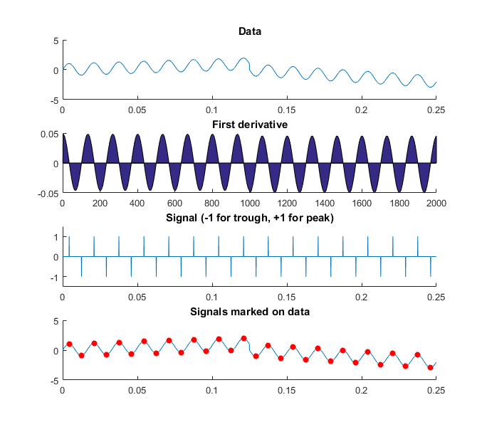
This yields:

This method will work extremely well for any type of sinusoid, with the only requirement that the input signal contains no noise.

---

Case 2: sinusoid with noise

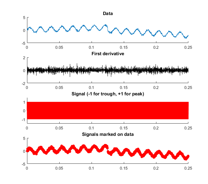
As soon as your input signal contains noise, the derivative method will fail. For example:

% Generate data
dt = 1/8000;
t  = (0:dt:(1-dt)/4)';
y  = sin(2*pi*60*t);

% Add some trends
y(1:1000) = y(1:1000) + 0.001*(1:1000)';
y(1001:2000) = y(1001:2000) - 0.002*(1:1000)';

% Add some noise
y = y + 0.2.*randn(2000,1);

Will now generate this result because first differences amplify noise:

Now there are many ways to deal with noise, and the most standard way is to apply a moving average filter. One disadvantage of moving averages is that they are slow to adapt to new information, such that signals may be identified after they have occurred (moving averages have a lag).

Another very typical approach is to use Fourier Analysis to identify all the frequencies in your input data, disregard all low-amplitude and high-frequency sinusoids, and use the remaining sinusoid as a filter. The remaining sinusoid will be (largely) cleansed from the noise and you can then use first-differencing again to determine the peaks and troughs (or for a single sine wave you know the peaks and troughs happen at 1/4 and 3/4 pi of the phase). I suggest you pick up any signal processing theory book to learn more about this technique. Matlab also has some educational material about this.

If you want to use this algorithm in hardware, I would suggest you also take a look at WFLC (Weighted Fourier Linear Combiner) with e.g. 1 oscillator or PLL (Phase-Locked Loop) that can estimate the phase of a noisy wave without doing a full Fast Fourier Transform. You can find a Matlab algorithm for a phase-locked loop on Wikipedia.

I will suggest a slightly more sophisticated approach here that will identify the peaks and troughs in real-time: fitting a sine wave function to your data using moving least squares minimization with initial estimates from Fourier analysis.

Here is my function to do that:

function [result, peaks, troughs] = fitsine(y, t, eps)

% Fast fourier-transform
f = fft(y);
l = length(y);
p2 = abs(f/l);
p1 = p2(1:ceil(l/2+1));
p1(2:end-1) = 2*p1(2:end-1);
freq = (1/mean(diff(t)))*(0:ceil(l/2))/l;

% Find maximum amplitude and frequency
maxPeak = p1 == max(p1(2:end)); % disregard 0 frequency!
maxAmplitude = p1(maxPeak);     % find maximum amplitude
maxFrequency = freq(maxPeak);   % find maximum frequency

% Initialize guesses
p = [];
p(1) = mean(y);         % vertical shift
p(2) = maxAmplitude;    % amplitude estimate
p(3) = maxFrequency;    % phase estimate
p(4) = 0;               % phase shift (no guess)
p(5) = 0;               % trend (no guess)

% Create model
f = @(p) p(1) + p(2)*sin( p(3)*2*pi*t+p(4) ) + p(5)*t;
ferror = @(p) sum((f(p) - y).^2);
% Nonlinear least squares
% If you have the Optimization toolbox, use [lsqcurvefit] instead!
options = optimset('MaxFunEvals',50000,'MaxIter',50000,'TolFun',1e-25);
[param,fval,exitflag,output] = fminsearch(ferror,p,options);

% Calculate result
result = f(param);

% Find peaks
peaks = abs(sin(param(3)*2*pi*t+param(4)) - 1) < eps;

% Find troughs
troughs = abs(sin(param(3)*2*pi*t+param(4)) + 1) < eps;

end

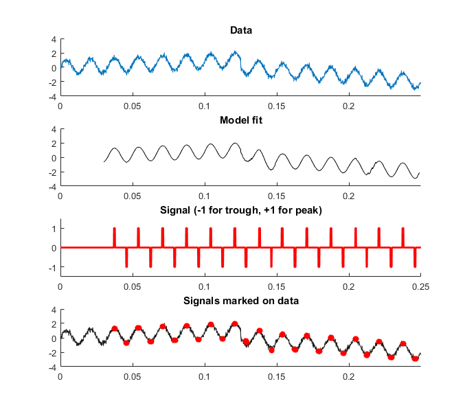
As you can see, I first perform a Fourier transform to find initial estimates of the amplitude and frequency of the data. I then fit a sinusoid to the data using the model a + b sin(ct + d) + et. The fitted values represent a sine wave of which I know that +1 and -1 are the peaks and troughs, respectively. I can therefore identify these values as the signals.

This works very well for sinusoids with (slowly changing) trends and general (white) noise:

% Generate data
dt = 1/8000;
t  = (0:dt:(1-dt)/4)';
y  = sin(2*pi*60*t);

% Add some trends
y(1:1000) = y(1:1000) + 0.001*(1:1000)';
y(1001:2000) = y(1001:2000) - 0.002*(1:1000)';

% Add some noise
y = y + 0.2.*randn(2000,1);

% Loop through data (moving window) and fit sine wave
window = 250;   % How many data points to consider
interval = 10;  % How often to estimate
result = nan(size(y));
signal = zeros(size(y));
for i = window+1:interval:length(y)
    data = y(i-window:i);   % Get data window
    period = t(i-window:i); % Get time window
    [output, peaks, troughs] = fitsine(data,period,0.01);
    
    result(i-interval:i) = output(end-interval:end);
    signal(i-interval:i) = peaks(end-interval:end) - troughs(end-interval:end);
end

% Plot result
figure(1); clf; set(gcf,'Position',[0 0 677 600])
subplot(4,1,1); hold on;
title('Data');
plot(t,y); xlim([0 max(t)]); ylim([-4 4]);
subplot(4,1,2); hold on;
title('Model fit');
plot(t,result,'-k'); xlim([0 max(t)]); ylim([-4 4]);
subplot(4,1,3); hold on;
title('Signal (-1 for trough, +1 for peak)');
plot(t,signal,'r','LineWidth',2); ylim([-1.5 1.5]);
subplot(4,1,4); hold on;
title('Signals marked on data');
markers = abs(signal) > 0;
plot(t,y,'-','Color',[0.1 0.1 0.1]);
scatter(t(markers),result(markers),30,'or','MarkerFaceColor','red');
xlim([0 max(t)]); ylim([-4 4]);

Main advantages of this approach are:

• You have an actual model of your data, so you can predict signals in the future before they happen! (e.g. fix the model and calculate the result by inputting future time periods)
• You don't need to estimate the model every period (see parameter interval in the code)

The disadvantage is that you need to select a lookback window, but you will have this problem with any method that you use for real-time detection.

Video demonstration

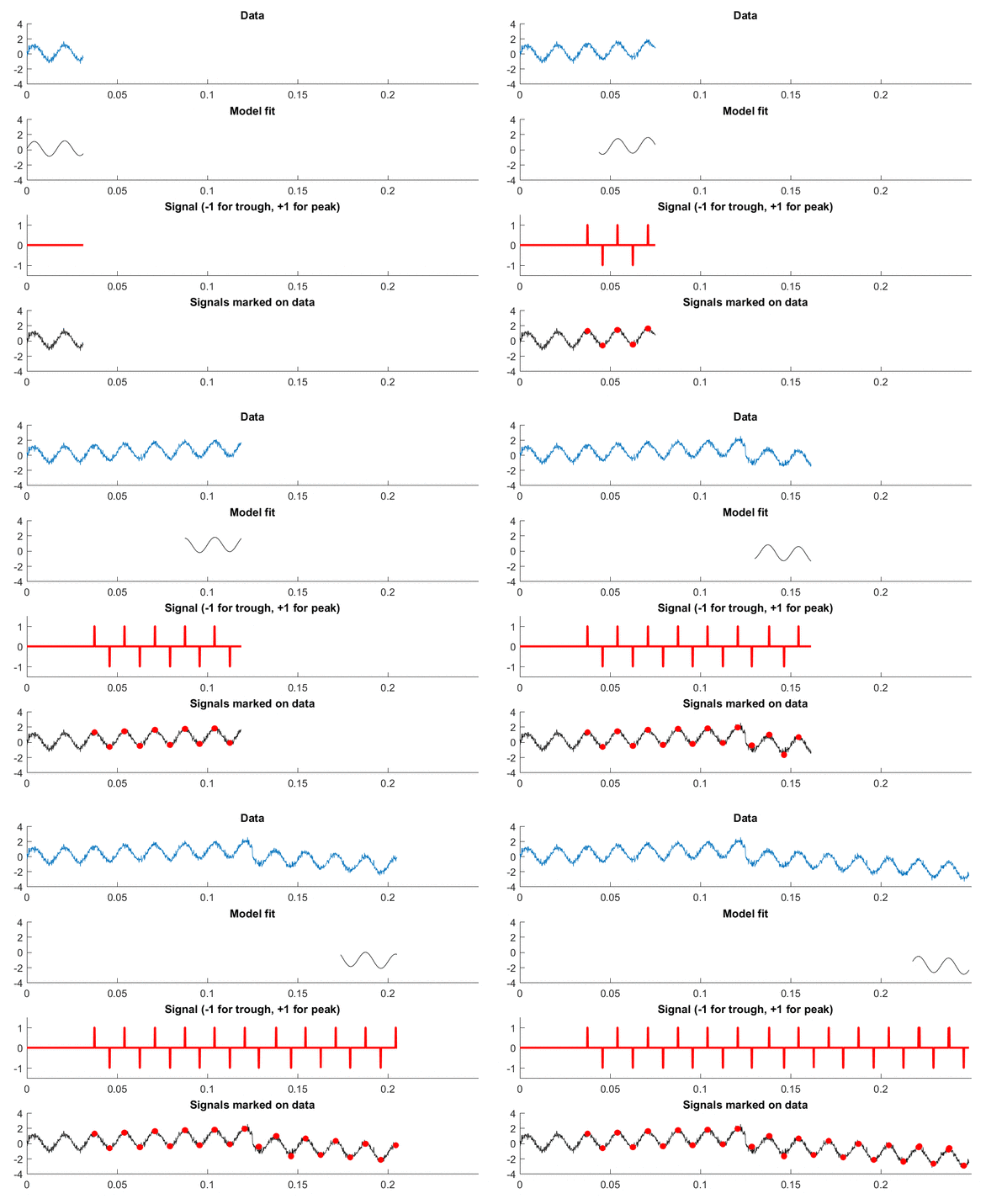
Data is the input data, Model fit is the fitted sine wave to the data (see code), Signal indicates the peaks and troughs and Signals marked on data gives an impression of how accurate the algorithm is. Note: watch the model fit adjust itself to the trend in the middle of the graph!

That should get you started. There are also a lot of excellent books on signal detection theory (just google that term), which will go much further into these types of techniques. Good luck!

Clavus

Answer 2

Consider using findpeaks, it is fast, which may be important for realtime. You should filter high-frequency noise to improve accuracy. here I smooth the data with a moving window.

t = 0:0.001:10;
x = 0.3*sin(t) + sin(1.3*t) + 0.9*sin(4.2*t) + 0.02*randn(1, 10001);
[~,iPeak0] = findpeaks(movmean(x,100),'MinPeakProminence',0.5);

You can time the process (0.0015sec)

f0 = @() findpeaks(movmean(x,100),'MinPeakProminence',0.5)
disp(timeit(f0,2))

To compare, processing the slope is only a bit faster (0.00013sec), but findpeaks have many useful options, such as minimum interval between peaks etc.

iPeaks1 = derivePeaks(x);
f1 = @() derivePeaks(x)
disp(timeit(f1,1))

Where derivePeaks is:

function iPeak1 = derivePeaks(x)
xSmooth = movmean(x,100);
goingUp = find(diff(movmean(xSmooth,100)) > 0);
iPeak1 = unique(goingUp([1,find(diff(goingUp) > 100),end]));
iPeak1(iPeak1 == 1 | iPeak1 == length(iPeak1)) = [];
end

Naamann