Understanding output from statsmodels grangercausalitytests

Question

I'm new to Granger Causality and would appreciate any advice on understanding/interpreting the results of the python statsmodels output. I've constructed two data sets (sine functions shifted in time with noise added)

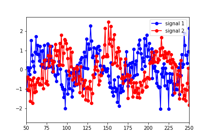
and put them in a "data" matrix with signal 1 as the first column and signal 2 as the second. I then ran the tests using:

granger_test_result = sm.tsa.stattools.grangercausalitytests(data, maxlag=40, verbose=True)`

The results showed that the optimal lag (in terms of the highest F test value) were for a lag of 1.

Granger Causality
('number of lags (no zero)', 1)
ssr based F test:         F=96.6366 , p=0.0000  , df_denom=995, df_num=1
ssr based chi2 test:   chi2=96.9280 , p=0.0000  , df=1
likelihood ratio test: chi2=92.5052 , p=0.0000  , df=1
parameter F test:         F=96.6366 , p=0.0000  , df_denom=995, df_num=1

However, the lag that seems to best describe the optimal overlap of the data is around 25 (in the figure below, signal 1 has been shifted to the right by 25 points):

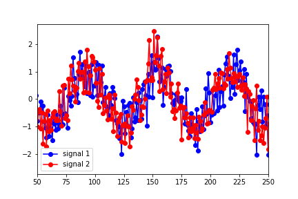
Granger Causality
('number of lags (no zero)', 25)
ssr based F test:         F=4.1891  , p=0.0000  , df_denom=923, df_num=25
ssr based chi2 test:   chi2=110.5149, p=0.0000  , df=25
likelihood ratio test: chi2=104.6823, p=0.0000  , df=25
parameter F test:         F=4.1891  , p=0.0000  , df_denom=923, df_num=25

I'm clearly misinterpreting something here. Why wouldn't the predicted lag match up with the shift in the data?

Also, can anyone explain to me why the p-values are so small as to be negligible for most lag values? They only begin to show up as non-zero for lags greater than 30.

Thanks for any help you can give.

Thurber

Could you find an answer to this? – Hayfork

What is the causal structure you're aiming to detect in your example? It seems like you're expecting to maximise cross-correlation. – Lachellelaches

Answer 1

As stated here, in order to run a Granger Causality test, the time series' you are using must be stationary. A common way to achieve this is to transform both series by taking the first difference of each:

x = np.diff(x)[1:]
y = np.diff(y)[1:]

Here is the comparison of Granger Causality results at lag 1 and lag 25 for the similar dataset I generated:

Unchanged

Granger Causality
number of lags (no zero) 1
ssr based F test:         F=19.8998 , p=0.0000  , df_denom=221, df_num=1
ssr based chi2 test:   chi2=20.1700 , p=0.0000  , df=1
likelihood ratio test: chi2=19.3129 , p=0.0000  , df=1
parameter F test:         F=19.8998 , p=0.0000  , df_denom=221, df_num=1

Granger Causality
number of lags (no zero) 25
ssr based F test:         F=6.9970  , p=0.0000  , df_denom=149, df_num=25
ssr based chi2 test:   chi2=234.7975, p=0.0000  , df=25
likelihood ratio test: chi2=155.3126, p=0.0000  , df=25
parameter F test:         F=6.9970  , p=0.0000  , df_denom=149, df_num=25

1st Difference

Granger Causality
number of lags (no zero) 1
ssr based F test:         F=0.1279  , p=0.7210  , df_denom=219, df_num=1
ssr based chi2 test:   chi2=0.1297  , p=0.7188  , df=1
likelihood ratio test: chi2=0.1296  , p=0.7188  , df=1
parameter F test:         F=0.1279  , p=0.7210  , df_denom=219, df_num=1

Granger Causality
number of lags (no zero) 25
ssr based F test:         F=6.2471  , p=0.0000  , df_denom=147, df_num=25
ssr based chi2 test:   chi2=210.3621, p=0.0000  , df=25
likelihood ratio test: chi2=143.3297, p=0.0000  , df=25
parameter F test:         F=6.2471  , p=0.0000  , df_denom=147, df_num=25

I'll try to explain what is happening conceptually. Due to the series you are using having a clear trend in mean, the early lags at 1, 2, ... etc. all give significant predictive models in the F test. This is because you can negatively correlate the x values 1 lag a way with the y values very easily, due to the long term trend. Additionally (this one is more of an educated guess), I think the reason you see the F statistic for lag 25 very low compared to the early lags is that a lot of the variance explained by the x series is contained in the auto-correlation of y from lags 1-25, since the non-stationarity gives the auto correlation more predictive power.

Pita

Hi @rsmith49, from what I read and see above the timeseries in question are sine waves with some noise added, how would these be non-stationary? – Carrel

Honestly this sent me down a bit of a rabbit hole, since my experience with time series was one grad class and then a bit of investigation for work. But looks like from here that Strict Sense Stationarity would exclude a sine wave plus noise. I'm assuming, based on the results from my experiment, that Granger Causality tests require Strict Sense Stationarity – Pita

@Carrel - the sine wave with noise isn't Weak Sense or Strict Sense Stationary: a necessary condition is that the mean of the distribution, m(t), needs to be the same for all times t and any shifts s. That is m(t + s) = m(t) for all s, t. This is true of the first differences if white noise was added to the sines, but is not true of the raw series plotted by the OP: m(t) is a sine function. – Lachellelaches

Answer 2

From the notes of the statsmodels.tsa.stattools.grangercausalitytests function

The Null hypothesis for grangercausalitytests is that the time series in the second column, x2, does NOT Granger cause the time series in the first column, x1. Grange causality means that past values of x2 have a statistically significant effect on the current value of x1, taking past values of x1 into account as regressors. We reject the null hypothesis that x2 does not Granger cause x1 if the pvalues are below a desired size of the test.

The null hypothesis for all four test is that the coefficients corresponding to past values of the second time series are zero.

the test is working exactly as expected.

Let's fix a significance level for your test, say alpha = 5% or 1%. It is important to choose it before performing the test. Then you run your Granger (non-)causality test, whose null hypothesis is that the second time series doesn't cause the first one, in the sense of Granger, for a fixed lag. As you found, the pvalue for lag = 1 is higher than the threshold alpha that you fixed, meaning that you can reject the null hypothesis (i.e. no causation). For lag > 25 the pvalues drop to zero, meaning that you should reject the null hypothesis, that is non-causation.

This is indeed in agreement with what you provided as time series by construction.

Douai

Answer 3

Did anyone mention the premise in the original question was incorrect?

"The results showed that the optimal lag (in terms of the highest F test value) were for a lag of 1. ..."

... that statement is incorrect. The F-values and chi2 come from different dof. The first lag model always has df=1. That yields a different distribution of test scores to when df=25.

You cannot compare F-test or chi2 scores for different degrees of freedom, since they'll have different distributions. You compare p-values instead, or better, as @AstoundingJB notes, choose a cut-off alpha and ignore the p-value value, only look at the binary decision that it is less than or greater than alpha. Or choose a range of alpha, and if the p-value is in the middle conclude the test is inconclusive.

Also the methodology suggested by @rsmith49 is the way to go: remove the long term trends by taking a first difference. But you should check (at least by plotting) this does make the time series "stationary". If there is still a trend do another differencing or in the raw data manually subtract off a curve fit - but if you find you have to do that it is questionable that a Granger test is useful, you might want to also try VAR tests: (https://en.wikipedia.org/wiki/Vector_autoregression

Busload