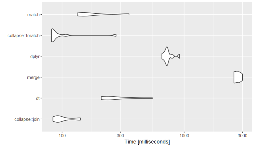
The match approach works when there is a unique key in the second data frame for each key value in the first. If there are duplicates in the second data frame then the match and merge approaches are not the same. Match is, of course, faster since it is not doing as much. In particular it never looks for duplicate keys. (continued after code)
DF1 = data.frame(a = c(1, 1, 2, 2), b = 1:4)
DF2 = data.frame(b = c(1, 2, 3, 3, 4), c = letters[1:5])
merge(DF1, DF2)
    b a c
  1 1 1 a
  2 2 1 b
  3 3 2 c
  4 3 2 d
  5 4 2 e
DF1$c = DF2$c[match(DF1$b, DF2$b)]
DF1$c
[1] a b c e
Levels: a b c d e

> DF1
  a b c
1 1 1 a
2 1 2 b
3 2 3 c
4 2 4 e
In the sqldf code that was posted in the question, it might appear that indexes were used on the two tables but, in fact, they are placed on tables which were overwritten before the sql select ever runs and that, in part, accounts for why its so slow. The idea of sqldf is that the data frames in your R session constitute the data base, not the tables in sqlite. Thus each time the code refers to an unqualified table name it will look in your R workspace for it -- not in sqlite's main database. Thus the select statement that was shown reads d1 and d2 from the workspace into sqlite's main database clobbering the ones that were there with the indexes. As a result it does a join with no indexes. If you wanted to make use of the versions of d1 and d2 that were in sqlite's main database you would have to refer to them as main.d1 and main.d2 and not as d1 and d2. Also, if you are trying to make it run as fast as possible then note that a simple join can't make use of indexes on both tables so you can save the time of creating one of the indexes. In the code below we illustrate these points.
Its worthwhile to notice that the precise computation can make a huge difference on which package is fastest. For example, we do a merge and an aggregate below. We see that the results are nearly reversed for the two. In the first example from fastest to slowest we get: data.table, plyr, merge and sqldf whereas in the second example sqldf, aggregate, data.table and plyr -- nearly the reverse of the first one. In the first example sqldf is 3x slower than data.table and in the second its 200x faster than plyr and 100 times faster than data.table. Below we show the input code, the output timings for the merge and the output timings for the aggregate. Its also worthwhile noting that sqldf is based on a database and therefore can handle objects larger than R can handle (if you use the dbname argument of sqldf) while the other approaches are limited to processing in main memory. Also we have illustrated sqldf with sqlite but it also supports the H2 and PostgreSQL databases as well.
library(plyr)
library(data.table)
library(sqldf)

set.seed(123)
N <- 1e5
d1 <- data.frame(x=sample(N,N), y1=rnorm(N))
d2 <- data.frame(x=sample(N,N), y2=rnorm(N))

g1 <- sample(1:1000, N, replace = TRUE)
g2<- sample(1:1000, N, replace = TRUE)
d <- data.frame(d1, g1, g2)

library(rbenchmark)

benchmark(replications = 1, order = "elapsed",
   merge = merge(d1, d2),
   plyr = join(d1, d2),
   data.table = {
      dt1 <- data.table(d1, key = "x")
      dt2 <- data.table(d2, key = "x")
      data.frame( dt1[dt2,list(x,y1,y2=dt2$y2)] )
      },
   sqldf = sqldf(c("create index ix1 on d1(x)",
      "select * from main.d1 join d2 using(x)"))
)

set.seed(123)
N <- 1e5
g1 <- sample(1:1000, N, replace = TRUE)
g2<- sample(1:1000, N, replace = TRUE)
d <- data.frame(x=sample(N,N), y=rnorm(N), g1, g2)

benchmark(replications = 1, order = "elapsed",
   aggregate = aggregate(d[c("x", "y")], d[c("g1", "g2")], mean),
   data.table = {
      dt <- data.table(d, key = "g1,g2")
      dt[, colMeans(cbind(x, y)), by = "g1,g2"]
   },
   plyr = ddply(d, .(g1, g2), summarise, avx = mean(x), avy=mean(y)),
   sqldf = sqldf(c("create index ix on d(g1, g2)",
      "select g1, g2, avg(x), avg(y) from main.d group by g1, g2"))
)
The outputs from the two benchmark call comparing the merge calculations are:
Joining by: x
        test replications elapsed relative user.self sys.self user.child sys.child
3 data.table            1    0.34 1.000000      0.31     0.01         NA        NA
2       plyr            1    0.44 1.294118      0.39     0.02         NA        NA
1      merge            1    1.17 3.441176      1.10     0.04         NA        NA
4      sqldf            1    3.34 9.823529      3.24     0.04         NA        NA
The output from the benchmark call comparing the aggregate calculations are:
        test replications elapsed  relative user.self sys.self user.child sys.child
4      sqldf            1    2.81  1.000000      2.73     0.02         NA        NA
1  aggregate            1   14.89  5.298932     14.89     0.00         NA        NA
2 data.table            1  132.46 47.138790    131.70     0.08         NA        NA
3       plyr            1  212.69 75.690391    211.57     0.56         NA        NA

