How to plot the survival curve generated by survreg (package survival of R)?
Asked Answered
C

5

37

I’m trying to fit and plot a Weibull model to a survival data. The data has just one covariate, cohort, which runs from 2006 to 2010. So, any ideas on what to add to the two lines of code that follows to plot the survival curve of the cohort of 2010?

library(survival)
s <- Surv(subSetCdm$dur,subSetCdm$event)
sWei <- survreg(s ~ cohort,dist='weibull',data=subSetCdm)

Accomplishing the same with the Cox PH model is rather straightforward, with the following lines. The problem is that survfit() doesn’t accept objects of type survreg.

sCox <- coxph(s ~ cohort,data=subSetCdm)
cohort <- factor(c(2010),levels=2006:2010)
sfCox <- survfit(sCox,newdata=data.frame(cohort))
plot(sfCox,col='green')

Using the data lung (from the survival package), here is what I'm trying to accomplish.

#create a Surv object
s <- with(lung,Surv(time,status))

#plot kaplan-meier estimate, per sex
fKM <- survfit(s ~ sex,data=lung)
plot(fKM)

#plot Cox PH survival curves, per sex
sCox <- coxph(s ~ as.factor(sex),data=lung)
lines(survfit(sCox,newdata=data.frame(sex=1)),col='green')
lines(survfit(sCox,newdata=data.frame(sex=2)),col='green')

#plot weibull survival curves, per sex, DOES NOT RUN
sWei <- survreg(s ~ as.factor(sex),dist='weibull',data=lung)
lines(survfit(sWei,newdata=data.frame(sex=1)),col='red')
lines(survfit(sWei,newdata=data.frame(sex=2)),col='red')
Curbstone answered 5/2, 2012 at 18:2 Comment(2)
I'd try to figure it out for ya if you posted a full example. We need the subSetCdm object. try dput(subSetCdm)Bourdon
There are examples in ?predict.survreg.Meyers
B
26

Hope this helps and I haven't made some misleading mistake:

copied from above:

    #create a Surv object
    s <- with(lung,Surv(time,status))

    #plot kaplan-meier estimate, per sex
    fKM <- survfit(s ~ sex,data=lung)
    plot(fKM)

    #plot Cox PH survival curves, per sex
    sCox <- coxph(s ~ as.factor(sex),data=lung)
    lines(survfit(sCox,newdata=data.frame(sex=1)),col='green')
    lines(survfit(sCox,newdata=data.frame(sex=2)),col='green')

for Weibull, use predict, re the comment from Vincent:

    #plot weibull survival curves, per sex,
    sWei <- survreg(s ~ as.factor(sex),dist='weibull',data=lung)

    lines(predict(sWei, newdata=list(sex=1),type="quantile",p=seq(.01,.99,by=.01)),seq(.99,.01,by=-.01),col="red")
    lines(predict(sWei, newdata=list(sex=2),type="quantile",p=seq(.01,.99,by=.01)),seq(.99,.01,by=-.01),col="red")

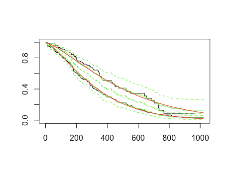
plot output

The trick here was reversing the quantile orders for plotting vs predicting. There is likely a better way to do this, but it works here. Good luck!

Bourdon answered 6/2, 2012 at 20:48 Comment(5)
Tim, quick question. If you wanted to recreate the above but NOT subset by gender... for example start with-- sWei <- survreg(s ~ 1,dist='weibull',data=lung). How would you change your specification of the newdata portion of your predict function? I'm trying to grok how you specified that in the above...Biskra
Hi Chris, I'm stumped, sorry, but perhaps one of the other answerers knows. If not, then maybe a new question.Bourdon
Considering your trick, reversing the sequence of quantiles (I'll call it q.seq here): If I understand it correctly, predict expects death quantiles, not survival. Therefore, I think it is better to supply 1 - q.seq instead of rev(q.seq). In your case it doesn't matter, because your q.seq is symmetrical, going from 0.01 death probability (= 0.99 survival) to 0.99 (= 0.01 survival). But it would make a difference if you went from, say, 0.01 to 0.8 death probability: your complementary sequence should be 0.99...0.2, and NOT 0.8 to 0.01.Biologist
I expanded on Igor's comment here: https://mcmap.net/q/415959/-how-to-plot-the-survival-curve-generated-by-survreg-package-survival-of-rFactorage
predict’s output depends on the “type” parameter. See ?predict.coxphAble
B
19

An alternative option is to make use of the package flexsurv. This offers some additional functionality over the survival package - including that the parametric regression function flexsurvreg() has a nice plot method which does what you ask.

Using lung as above;

#create a Surv object
s <- with(lung,Surv(time,status))

require(flexsurv)
sWei  <- flexsurvreg(s ~ as.factor(sex),dist='weibull',data=lung)
sLno  <- flexsurvreg(s ~ as.factor(sex),dist='lnorm',data=lung)   

plot(sWei)
lines(sLno, col="blue")

output from plot.flexsurvreg

You can plot on the cumulative hazard or hazard scale using the type argument, and add confidence intervals with the ci argument.

Basketry answered 14/3, 2014 at 13:55 Comment(0)
F
10

This is just a note clarifying Tim Riffe's answer, which uses the following code:

lines(predict(sWei, newdata=list(sex=1),type="quantile",p=seq(.01,.99,by=.01)),seq(.99,.01,by=-.01),col="red")
lines(predict(sWei, newdata=list(sex=2),type="quantile",p=seq(.01,.99,by=.01)),seq(.99,.01,by=-.01),col="red")

The reason for the two mirror-image sequences, seq(.01,.99,by=.01) and seq(.99,.01,by=-.01), is because the predict() method is giving quantiles for the event distribution f(t) - that is, values of the inverse CDF of f(t) - while a survival curve is plotting 1-(CDF of f) versus t. In other words, if you plot p versus predict(p), you'll get the CDF, and if you plot 1-p versus predict(p) you'll get the survival curve, which is 1-CDF. The following code is more transparent and generalizes to arbitrary vectors of p values:

pct <- seq(.01,.99,by=.01)
lines(predict(sWei, newdata=list(sex=1),type="quantile",p=pct),1-pct,col="red")
lines(predict(sWei, newdata=list(sex=2),type="quantile",p=pct),1-pct,col="red")
Factorage answered 13/5, 2015 at 12:51 Comment(0)
L
3

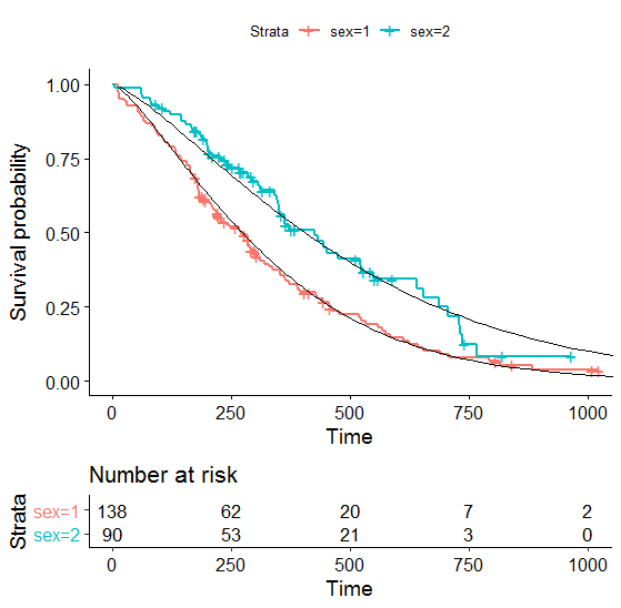
In case someone wants to add a Weibull distribution to the Kaplan-Meyer curve in the ggplot2 ecosystem, we can do the following:

library(survminer)
library(tidyr)

s <- with(lung,Surv(time,status))
fKM <- survfit(s ~ sex,data=lung)
sWei <- survreg(s ~ as.factor(sex),dist='weibull',data=lung)

pred.sex1 = predict(sWei, newdata=list(sex=1),type="quantile",p=seq(.01,.99,by=.01))
pred.sex2 = predict(sWei, newdata=list(sex=2),type="quantile",p=seq(.01,.99,by=.01))

df = data.frame(y=seq(.99,.01,by=-.01), sex1=pred.sex1, sex2=pred.sex2)
df_long = gather(df, key= "sex", value="time", -y)

p = ggsurvplot(fKM, data = lung, risk.table = T)
p$plot = p$plot + geom_line(data=df_long, aes(x=time, y=y, group=sex))

enter image description here

Ladino answered 27/5, 2020 at 14:41 Comment(0)
E
1

In case you'd like to use the survival function itself S(t) (instead of the inverse survival function S^{-1}(p) used in other answers here) I've written a function to implement that for the case of the Weibull distribution (following the same inputs as the pec::predictSurvProb family of functions:

survreg.predictSurvProb <- function(object, newdata, times){
  shape <- 1/object$scale # also equals 1/exp(fit$icoef[2])
  lps <- predict(object, newdata = newdata, type = "lp")
  surv <- t(sapply(lps, function(lp){
    sapply(times, function(t) 1 - pweibull(t, shape = shape, scale = exp(lp)))
  }))
  
  return(surv)
}

You can then do:

sWei <- survreg(s ~ as.factor(sex),dist='weibull',data=lung)
times <- seq(min(lung$time), max(lung$time), length.out = 1000)
new_dat <- data.frame(sex = c(1,2))
surv <- survreg.predictSurvProb(sWei, newdata = new_dat, times = times)

lines(times, surv[1, ],col='red')
lines(times, surv[2, ],col='red')

enter image description here

Excommunicate answered 12/6, 2020 at 7:19 Comment(0)

© 2022 - 2024 — McMap. All rights reserved.