Plot trees for a Random Forest in Python with Scikit-Learn

Question

I want to plot a decision tree of a random forest. So, i create the following code:

clf = RandomForestClassifier(n_estimators=100)
import pydotplus
import six
from sklearn import tree
dotfile = six.StringIO()
i_tree = 0
for tree_in_forest in clf.estimators_:
if (i_tree <1):        
    tree.export_graphviz(tree_in_forest, out_file=dotfile)
    pydotplus.graph_from_dot_data(dotfile.getvalue()).write_png('dtree'+ str(i_tree) +'.png')
    i_tree = i_tree + 1

But it doesn't generate anything.. Have you an idea how to plot a decision tree from random forest?

Blanche

Answer 1

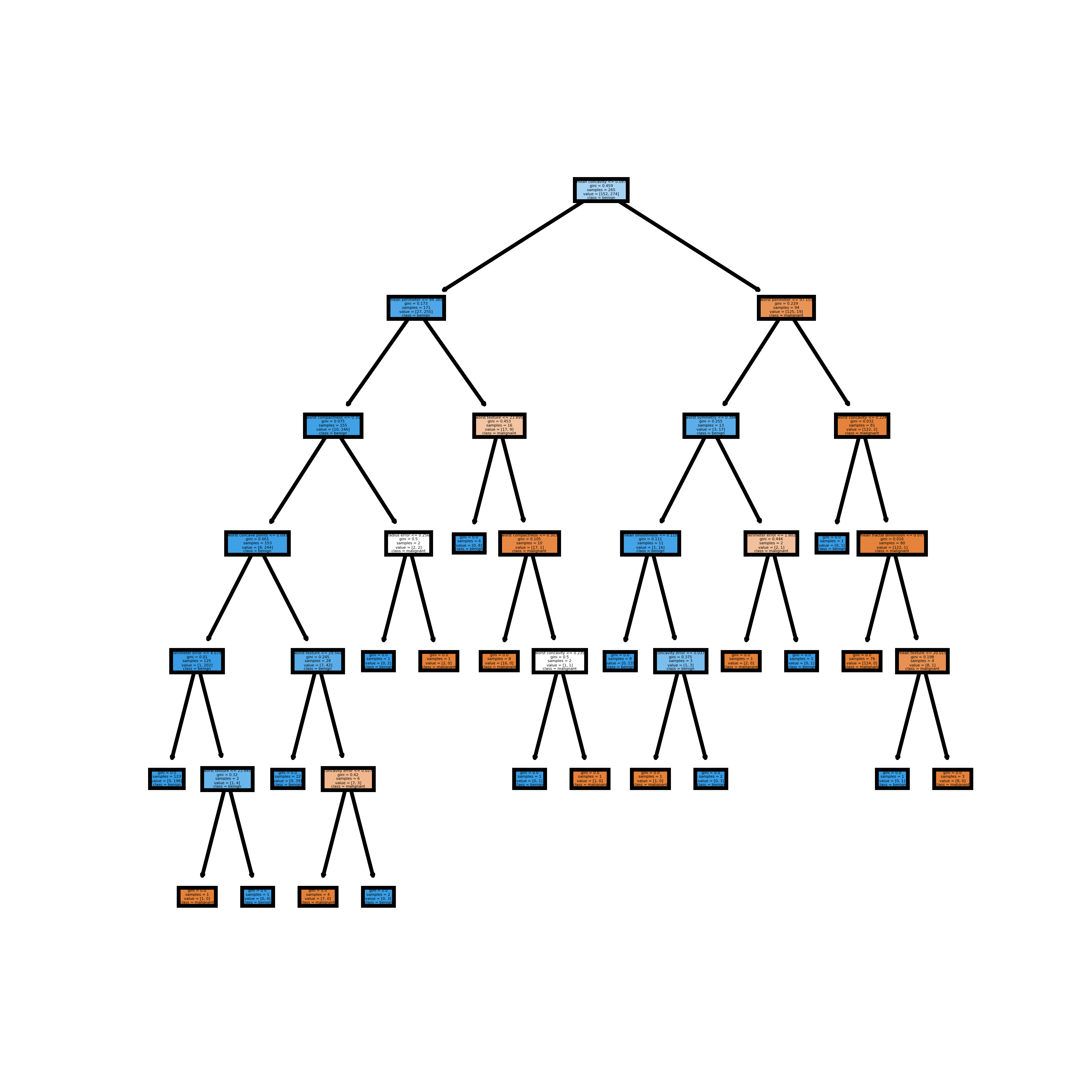
After you fit a random forest model in scikit-learn, you can visualize individual decision trees from a random forest. The code below first fits a random forest model.

import matplotlib.pyplot as plt
from sklearn.datasets import load_breast_cancer
from sklearn import tree
import pandas as pd
from sklearn.ensemble import RandomForestClassifier
from sklearn.model_selection import train_test_split

# Load the Breast Cancer Dataset
data = load_breast_cancer()
df = pd.DataFrame(data.data, columns=data.feature_names)
df['target'] = data.target

# Arrange Data into Features Matrix and Target Vector
X = df.loc[:, df.columns != 'target']
y = df.loc[:, 'target'].values

# Split the data into training and testing sets
X_train, X_test, Y_train, Y_test = train_test_split(X, y, random_state=0)

# Random Forests in `scikit-learn` (with N = 100)
rf = RandomForestClassifier(n_estimators=100,
                            random_state=0)
rf.fit(X_train, Y_train)

You can now visualize individual trees. The code below visualizes the first decision tree.

fn=data.feature_names
cn=data.target_names
fig, axes = plt.subplots(nrows = 1,ncols = 1,figsize = (4,4), dpi=800)
tree.plot_tree(rf.estimators_[0],
               feature_names = fn, 
               class_names=cn,
               filled = True);
fig.savefig('rf_individualtree.png')

The image below is what is saved.

Because this question asked for trees, you can visualize all the estimators (decision trees) from a random forest if you like. The code below visualizes the first 5 from the random forest model fit above.

# This may not the best way to view each estimator as it is small
fn=data.feature_names
cn=data.target_names
fig, axes = plt.subplots(nrows = 1,ncols = 5,figsize = (10,2), dpi=900)
for index in range(0, 5):
    tree.plot_tree(rf.estimators_[index],
                   feature_names = fn, 
                   class_names=cn,
                   filled = True,
                   ax = axes[index]);

    axes[index].set_title('Estimator: ' + str(index), fontsize = 11)
fig.savefig('rf_5trees.png')

The image below is what is saved.

The code was adapted from this post.

Scarper

Answer 2

Assuming your Random Forest model is already fitted, first you should first import the export_graphviz function:

from sklearn.tree import export_graphviz

In your for cycle you could do the following to generate the dot file

export_graphviz(tree_in_forest,
                feature_names=X.columns,
                filled=True,
                rounded=True)

The next line generates a png file

os.system('dot -Tpng tree.dot -o tree.png')

Hyrup

I think there is no attribute of tree in random forest, isn't it? – Lundt

@LKM, a Random Forest is a list of trees. You can get that list using the estimators_ attribute. You can export for example the first tree using random_forest.estimators_[0]. – Reneerenegade

"export_graphviz" can be used only for decision trees but not Random Forests. – Hirza

@Lundt a tree is an element of the list clf.estimators_ – Hyrup

len(random_forest.estimators_) gives the number of trees. – Osteal

Answer 3

To access the single decision tree from the random forest in scikit-learn use estimators_ attribute:

rf = RandomForestClassifier()
# first decision tree
rf.estimators_[0]

Then you can use standard way to visualize the decision tree:

• you can print the tree representation, with sklearn export_text
• export to graphiviz and plot with sklearn export_graphviz method
• plot with matplotlib with sklearn plot_tree method
• use dtreeviz package for tree plotting

The code with example output are described in this post.

The important thing to while plotting the single decision tree from the random forest is that it might be fully grown (default hyper-parameters). It means the tree can be really depth. For me, the tree with depth greater than 6 is very hard to read. So if the tree visualization will be needed I'm building random forest with max_depth < 7. You can check the example visualization in this post.

Shcherbakov

Answer 4

you can view each tree like this,

i_tree = 0
for tree_in_forest in FT_cls_gini.estimators_:
    if (i_tree ==3):        
        tree.export_graphviz(tree_in_forest, out_file=dotfile)
        graph = pydotplus.graph_from_dot_data(dotfile.getvalue())        
    i_tree = i_tree + 1
Image(graph.create_png())

Slurry

Can you add some more explanation regarding how this is different from the other answers? Works better than just dumping code – Extensity

Answer 5

You can draw a single tree:

from sklearn.tree import export_graphviz
from IPython import display
from sklearn.ensemble import RandomForestRegressor

m = RandomForestRegressor(n_estimators=1, max_depth=3, bootstrap=False, n_jobs=-1)
m.fit(X_train, y_train)

str_tree = export_graphviz(m, 
   out_file=None, 
   feature_names=X_train.columns, # column names
   filled=True,        
   special_characters=True, 
   rotate=True, 
   precision=0.6)

display.display(str_tree)

Osteomalacia

Do you have idea what mean the parameters ratio and precision in the "draw_tree" function? – Agrestic

This method does not work anymore, because the .structured package has been removed from the library – Gigot

Answer 6

In addition to the solution given above, you can try this (hopefully for anyone that may need this in the future).

from sklearn.tree import export_graphviz
from six import StringIO 

i_tree = 0
dot_data = StringIO()
for tree_in_forest in rfc.estimators_:#rfc random forest classifier
    if (i_tree ==3):        
        export_graphviz(tree_in_forest, out_file=dot_data)
        graph = pydotplus.graph_from_dot_data(dot_data.getvalue())        
    i_tree = i_tree + 1
Image(graph.create_png())

Monia

Answer 7

I plot the random forest in IRIS dataset I think that might help you.

from sklearn.datasets import load_iris
from sklearn.ensemble import RandomForestClassifier
from sklearn import tree
import pydotplus
import os

# Load the Iris dataset for demonstration
iris = load_iris()
X = iris.data
y = iris.target

# Create a random forest classifier
clf = RandomForestClassifier(n_estimators=100)

# Train the classifier
clf.fit(X, y)

# Create directory to save decision tree images
os.makedirs("decision_trees", exist_ok=True)

# Plot decision trees of the random forest
for i, tree_in_forest in enumerate(clf.estimators_):
    dotfile = f"decision_trees/dtree_{i}.dot"
    pngfile = f"decision_trees/dtree_{i}.png"
    tree.export_graphviz(tree_in_forest, out_file=dotfile, feature_names=iris.feature_names, class_names=iris.target_names, filled=True, rounded=True)
    os.system(f"dot -Tpng {dotfile} -o {pngfile}")

Slaby