Inverting a real-valued index grid

Question

OpenCV's remap() uses a real-valued index grid to sample a grid of values from an image using bilinear interpolation, and returns the grid of samples as a new image.

To be precise, let:

A = an image 
X = a grid of real-valued X coords into the image. 
Y = a grid of real-valued Y coords into the image.
B = remap(A, X, Y)

Then for all pixel coordinates i, j,

B[i, j] = A(X[i, j], Y[i, j]) 

Where the round-braces notation A(x, y) denotes using bilinear interpolation to solve for the pixel value of image A using float-valued coords x and y.

My question is: given an index grid X, Y, how can I generate an "inverse grid" X^-1, Y^-1 such that:

X(X^-1[i, j], Y^-1[i, j]) = i
Y(X^-1[i, j], Y^-1[i, j]) = j

And

X^-1(X[i, j], Y[i, j]) = i
Y^-1(X[i, j], Y[i, j]) = j

For all integer pixel coordinates i, j?

FWIW, the image and index maps X and Y are the same shape. However, there is no a priori structure to the index maps X and Y. For example, they're not necessarily affine or rigid transforms. They may even be uninvertible, e.g. if X, Y maps multiple pixels in A to the same exact pixel coordinate in B. I'm looking for ideas for a method that will find a reasonable inverse map if one exists.

The solution need not be OpenCV-based, as I'm not using OpenCV, but another library that has a remap() implementation. While any suggestions are welcome, I'm particularly keen on something that's "mathematically correct", i.e. if my map M is perfectly invertible, the method should find the perfect inverse, within some small margin of machine precision.

Holography

Answer 1

This is an important problem, and I am surprised that it is not better addressed in any standard library (at least to my knowledge).

I wasn't happy with the accepted solution as it didn't use the implicit smoothness of the transformation. I might miss important cases, but I cannot imagine mapping that are both invertible in any useful sense and non-smooth at the pixel scale.

Smoothness means that there is no need to compute nearest neighbors: the nearest points are those that are already near on the original grid.

My solution uses the fact that, in the original mapping, a square [(i,j), (i+1, j), (i+1, j+1), (i, j+1)] maps to a quadrilateral [(X[i,j], Y[i,j], X[i+1,j], Y[i+1,j], ...] that has no other points inside. Then the inverse mapping only requires interpolation within the quadrilateral. For this I use an inverse bilinear interpolation, which will give exact results at the vertices and for any other affine transform.

The implementation has no other dependency than numpy. The logic is to run through all quadrilaterals and build progressively the reverse mapping. I copy the code here, hopefully there are enough comments to make the idea clear enough.

A few comments on the less obvious stuff:

• The inverse bilinear function would normally return coordinates only in the range [0,1]. I removed the clipping operation, so that out-of-range values mean that the coordinate is outside of the quadrilateral (that's a contorted way of solving the point-in-polygon problem!). To avoid missing points on the edges, I actually allow for points out of the [0,1] range, which normally means that an index may be picked up by two neighboring quadrilaterals. In these rare cases I just let the result be the average of the two result, trusting that the out-of-range points are "extrapolating" in a reasonable way.
• In general all quadrilaterals have a different shape, and their overlap with the regular grid can go from nothing at all to vary many points. The routine solves all quadrilateral at once (to exploit the vectorised nature of bilinear_inverse, but at each iteration selects only the quadrilaterals for which the coordinates (offset to their bounding box) are valid.

import numpy as np

def bilinear_inverse(p, vertices, numiter=4):
    """
    Compute the inverse of the bilinear map from the unit square
    [(0,0), (1,0), (1,1), (0,1)]
    to the quadrilateral vertices = [p0, p1, p2, p4]

    Parameters:
    ----------
    p: array of shape (2, ...)
        Points on which the inverse transforms are applied.
    vertices: array of shape (4, 2, ...)
        Coordinates of the vertices mapped to the unit square corners
    numiter:
        Number of Newton interations

    Returns:
    --------
    s: array of shape (2, ...)
        Mapped points.

    This is a (more general) python implementation of the matlab implementation 
    suggested in https://mcmap.net/q/380711/-inverse-bilinear-interpolation
    """

    p = np.asarray(p)
    v = np.asarray(vertices)
    sh = p.shape[1:]
    if v.ndim == 2:
        v = np.expand_dims(v, axis=tuple(range(2, 2 + len(sh))))

    # Start in the center
    s = .5 * np.ones((2,) + sh)
    s0, s1 = s
    for k in range(numiter):
        # Residual
        r = v[0] * (1 - s0) * (1 - s1) + v[1] * s0 * (1 - s1) + v[2] * s0 * s1 + v[3] * (1 - s0) * s1 - p

        # Jacobian
        J11 = -v[0, 0] * (1 - s1) + v[1, 0] * (1 - s1) + v[2, 0] * s1 - v[3, 0] * s1
        J21 = -v[0, 1] * (1 - s1) + v[1, 1] * (1 - s1) + v[2, 1] * s1 - v[3, 1] * s1
        J12 = -v[0, 0] * (1 - s0) - v[1, 0] * s0 + v[2, 0] * s0 + v[3, 0] * (1 - s0)
        J22 = -v[0, 1] * (1 - s0) - v[1, 1] * s0 + v[2, 1] * s0 + v[3, 1] * (1 - s0)

        inv_detJ = 1. / (J11 * J22 - J12 * J21)

        s0 -= inv_detJ * (J22 * r[0] - J12 * r[1])
        s1 -= inv_detJ * (-J21 * r[0] + J11 * r[1])

    return s


def invert_map(xmap, ymap, diagnostics=False):
    """
    Generate the inverse of deformation map defined by (xmap, ymap) using inverse bilinear interpolation.
    """

    # Generate quadrilaterals from mapped grid points.
    quads = np.array([[ymap[:-1, :-1], xmap[:-1, :-1]],
                      [ymap[1:, :-1], xmap[1:, :-1]],
                      [ymap[1:, 1:], xmap[1:, 1:]],
                      [ymap[:-1, 1:], xmap[:-1, 1:]]])

    # Range of indices possibly within each quadrilateral
    x0 = np.floor(quads[:, 1, ...].min(axis=0)).astype(int)
    x1 = np.ceil(quads[:, 1, ...].max(axis=0)).astype(int)
    y0 = np.floor(quads[:, 0, ...].min(axis=0)).astype(int)
    y1 = np.ceil(quads[:, 0, ...].max(axis=0)).astype(int)

    # Quad indices
    i0, j0 = np.indices(x0.shape)

    # Offset of destination map
    x0_offset = x0.min()
    y0_offset = y0.min()

    # Index range in x and y (per quad)
    xN = x1 - x0 + 1
    yN = y1 - y0 + 1

    # Shape of destination array
    sh_dest = (1 + x1.max() - x0_offset, 1 + y1.max() - y0_offset)

    # Coordinates of destination array
    yy_dest, xx_dest = np.indices(sh_dest)

    xmap1 = np.zeros(sh_dest)
    ymap1 = np.zeros(sh_dest)
    TN = np.zeros(sh_dest, dtype=int)

    # Smallish number to avoid missing point lying on edges
    epsilon = .01

    # Loop through indices possibly within quads
    for ix in range(xN.max()):
        for iy in range(yN.max()):
            # Work only with quads whose bounding box contain indices
            valid = (xN > ix) * (yN > iy)

            # Local points to check
            p = np.array([y0[valid] + ix, x0[valid] + iy])

            # Map the position of the point in the quad
            s = bilinear_inverse(p, quads[:, :, valid])

            # s out of unit square means p out of quad
            # Keep some epsilon around to avoid missing edges
            in_quad = np.all((s > -epsilon) * (s < (1 + epsilon)), axis=0)

            # Add found indices
            ii = p[0, in_quad] - y0_offset
            jj = p[1, in_quad] - x0_offset

            ymap1[ii, jj] += i0[valid][in_quad] + s[0][in_quad]
            xmap1[ii, jj] += j0[valid][in_quad] + s[1][in_quad]

            # Increment count
            TN[ii, jj] += 1

    ymap1 /= TN + (TN == 0)
    xmap1 /= TN + (TN == 0)

    if diagnostics:
        diag = {'x_offset': x0_offset,
                'y_offset': y0_offset,
                'mask': TN > 0}
        return xmap1, ymap1, diag
    else:
        return xmap1, ymap1

Here's a test example

import cv2 as cv
from scipy import ndimage as ndi

# Simulate deformation field
N = 500
sh = (N, N)
t = np.random.normal(size=sh)
dx = ndi.gaussian_filter(t, 40, order=(0,1))
dy = ndi.gaussian_filter(t, 40, order=(1,0))
dx *= 30/dx.max()
dy *= 30/dy.max()

# Test image
img = np.zeros(sh)
img[::10, :] = 1
img[:, ::10] = 1
img = ndi.gaussian_filter(img, 0.5)

# Apply forward mapping
yy, xx = np.indices(sh)
xmap = (xx-dx).astype(np.float32)
ymap = (yy-dy).astype(np.float32)
warped = cv.remap(img, xmap, ymap ,cv.INTER_LINEAR)
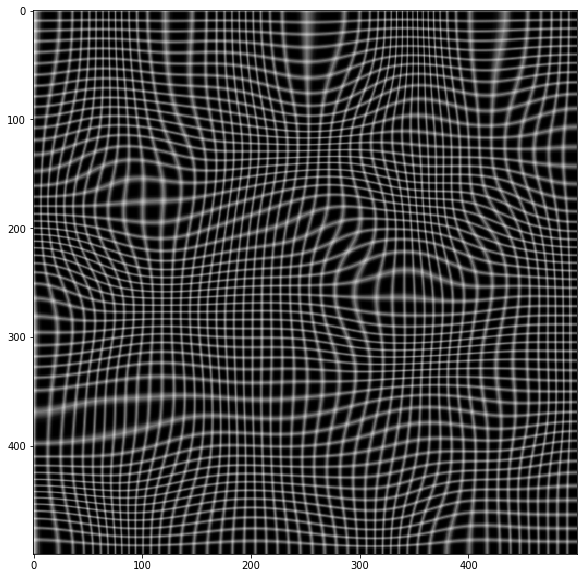
plt.imshow(warped, cmap='gray')

# Now invert the mapping
xmap1, ymap1 = invert_map(xmap, ymap)

unwarped = cv.remap(warped, xmap1.astype(np.float32), ymap1.astype(np.float32) ,cv.INTER_LINEAR)

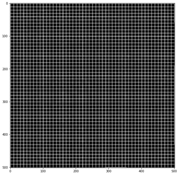
plt.imshow(unwarped, cmap='gray')

Inflammatory

bug in sh_dest = ..., order needs to be (height, width) -- code seems to be taking a good while to execute -- and it seems as if the resulting map contains spurious 0 indices (when needing to stretch the input)... i see hints of that in the last picture (result) – Zitazitah

Answer 2

Well I just had to solve this remap inversion problem myself and I'll outline my solution.

Given X, Y for the remap() function that does the following:

B[i, j] = A(X[i, j], Y[i, j])   

I computed Xinv, Yinv that can be used by the remap() function to invert the process:

A[x, y] = B(Xinv[x,y],Yinv[x,y])

First I build a KD-Tree for the 2D point set {(X[i,j],Y[i,j]} so I can efficiently find the N nearest neighbors to a given point (x,y). I use Euclidian distance for my distance metric. I found a great C++ header lib for KD-Trees on GitHub.

Then I loop thru all the (x,y) values in A's grid and find the N = 5 nearest neighbors {(X[i_k,j_k],Y[i_k,j_k]) | k = 0 .. N-1} in my point set.

• If distance d_k == 0 for some k then Xinv[x,y] = i_k and Yinv[x,y] = j_k, otherwise...

• Use Inverse Distance Weighting (IDW) to compute an interpolated value:

  • let weight w_k = 1 / pow(d_k, p) (I use p = 2)
  • Xinv[x,y] = (sum_k w_k * i_k)/(sum_k w_k)
  • Yinv[x,y] = (sum_k w_k * j_k)/(sum_k w_k)

Note that if B is a W x H image then X and Y are W x H arrays of floats. If A is a w x h image then Xinv and Yinv are w x h arrays for floats. It is important that you are consistent with image and map sizing.

Works like a charm! My first version I tried brute forcing the search and I never even waited for it to finish. I switched to a KD-Tree then I started to get reasonable run times. I f I ever get time I would like to add this to OpenCV.

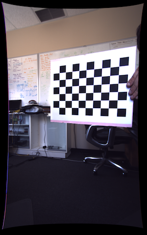
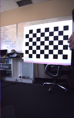
The second image below is use remap() to remove the lens distortion from the first image. The third image is a result of inverting the process.

Godding

Hi, can you share your code for this? I tried to implement but the result image didn't reverse the lens correction – Hedley

I've debugged the code and found the problem, thank you so much for your answer! – Hedley

@Hedley Glad it worked. I probably wold have posted a link to my code, but it is part of a larger project I can't share. I could extract the interesting part and post it, but it sounds like you got it. – Godding

Thx. I posted my implementation below, incase someone else might need it. – Hedley

You can find a python implementation of this clever idea here – Teneshatenesmus

I might be missing something, but this solution seems both arbitrary and wasteful. Arbitrariness: Why 5 neighbors? Why inverse distance weighting? Waste: why not use the grid structure to obtain the neighbors? The only meaningful applications are those where the mapping is both smooth and bijective, in which case no costly neighbor search is needed. – Inflammatory

@Inflammatory The points {(X[i,j],Y[i,j])} do not lie on a regular grid. In the case of radial lens distortion they lie on a grid that has been stretched like taffy (e.g., see second image in the corners). In other words, these points represent samples of a non-linear function -- when you have heavy fish-eye distortion and add tangential distortion you can forget using the grid to find neighbors. N = 5 neighbors is a nice goldilocks value -- not too few and not too many. IDW is a great way to interpolate a 2D surface sampled on a non regular grid. – Godding

I have just submitted my solution as an alternative answer. – Inflammatory

@Inflammatory Cool. I'll give it a go when I get a chance. Timing is interesting since I am currently working with modeling lens distortion again. – Godding

Answer 3

Iterative solution

Many of the above solutions didn't work for me, failed when the map wasn't invertible, or weren't terribly fast.

I present an alternative, 6-line iterative solution.

def invert_map(F):
    I = np.zeros_like(F)
    I[:,:,1], I[:,:,0] = np.indices(sh)
    P = np.copy(I)
    for i in range(10):
        P += I - cv.remap(F, P, None, interpolation=cv.INTER_LINEAR)
    return P

How well does it do? For my use case of inverting a terrain correction map for aerial photography, this method converges comfortably in 10 steps to 1/10th of a pixel. It's also blazingly fast, because all the heavy compute is tucked inside OpenCV

How does it work?

The approach uses the idea that if (x', y') = F(x, y) is a mapping, then the inverse can be approximated with (x, y) = -F(x', y'), as long as the gradient of F is small.

We can continue to refine our mapping, the above gets us our first prediction (I is an "identity mapping"):

G_1 = I - F

Our second prediction can be adapted from that:

G_2 = G_1 + I - F(G_1)

and so on:

G_n+1 = G_n + I - F(G_n)

Proving that G_n converges to the inverse F^-1 is hard, but what we can easily prove is that if G has converged, it will stay converged.

Assume G_n = F^-1, then we can substitute into:

G_n+1 = G_n + I - F(G_n)

and then get:

G_n+1 = F^-1 + I - F(F^-1)
G_n+1 = F^-1 + I - I
G_n+1 = F^-1
Q.E.D.

Testing script

import cv2 as cv
from scipy import ndimage as ndi
import numpy as np
from matplotlib import pyplot as plt

# Simulate deformation field
N = 500
sh = (N, N)
t = np.random.normal(size=sh)
dx = ndi.gaussian_filter(t, 40, order=(0,1))
dy = ndi.gaussian_filter(t, 40, order=(1,0))
dx *= 10/dx.max()
dy *= 10/dy.max()

# Test image
img = np.zeros(sh)
img[::10, :] = 1
img[:, ::10] = 1
img = ndi.gaussian_filter(img, 0.5)

# Apply forward mapping
yy, xx = np.indices(sh)
xmap = (xx-dx).astype(np.float32)
ymap = (yy-dy).astype(np.float32)
warped = cv.remap(img, xmap, ymap ,cv.INTER_LINEAR)
plt.imshow(warped, cmap='gray')

def invert_map(F: np.ndarray):
    I = np.zeros_like(F)
    I[:,:,1], I[:,:,0] = np.indices(sh)
    P = np.copy(I)
    for i in range(10):
        P += I - cv.remap(F, P, None, interpolation=cv.INTER_LINEAR)
    return P

# F: The function to invert
F = np.zeros((sh[0], sh[1], 2), dtype=np.float32)
F[:,:,0], F[:,:,1] = (xmap, ymap)

# Test the prediction
unwarped = cv.remap(warped, invert_map(F), None, cv.INTER_LINEAR)
plt.imshow(unwarped, cmap='gray')

Bahuvrihi

I like this because of its simplicity and solid mathematical foundation. – Zitazitah

remap limited precision because standard interpolation modes use fixed point math internally. it's limited to 5 fractional bits, AFAIK – Zitazitah

if the solution has trouble converging, or has large deviations near the edges of the image, which may be due to oscillations in the P += I - cv.remap(...) step, simply calculate P += (I - cv.remap(...)) * 0.5 instead. with that adjustment, the iteration is damped and converges within just 5-10 iterations (down to remap's fixed point numerical limits, which give you 5 fractional bits). – Zitazitah

Great answer. Wonderfully simple. In practice the forward map might be required to lose source data. Can you modify your answer to cope with this? This adjustment to the test code illustrates the point: Replace xmap = (xx-dx).astype(np.float32) with xmap = (0.1*N+xx*0.8-dx).astype(np.float32) We now see corruption down the left hand side of the image. And interestingly not the right hand side! Note, adding borderMode=cv.BORDER_CONSTANT, borderValue=0.5 to the cv.remap() line helps illustrate the the difference between the expected invalid pixels and any incorrect pixels. – Munich

Answer 4

You can invert map at known points and interpolate it into new grid. It will work fine, while distortion is not very huge.

Here is very simple implementation in Python using scipy.interpolate.griddata:

map_x, map_y = cv2.initUndistortRectifyMap(K, D, None, new_K, image_size, cv2.CV_32FC1)

points =  np.stack([map_x.flatten(), map_y.flatten()], axis=1)
grid = np.mgrid[:map_x.shape[0], :map_y.shape[1]]
values = grid.reshape(2, -1).T[..., ::-1] 

from scipy.interpolate import griddata
grid_y, grid_x = grid
map_back = griddata(points, values, (grid_x, grid_y), method='cubic').astype(map_undistort.dtype)

If you use CV_32FC2 for maps, you can simplify points construction:

map_undistort, _ = cv2.initUndistortRectifyMap(K, D, None, new_K, image_size, cv2.CV_32FC2)
points = map_undistort.reshape(-1, 2)

Amadoamador

Answer 5

If you map is derived from a homography H you could invert H and directly create the inverse maps with cv::initUndistortRectifyMap().

e.g. in Python:

import numpy as np.
map_size = () # fill in your map size
H_inv = np.linalg.inv(H)
map1, map2 = cv2.initUndistortRectifyMap(cameraMatrix=np.eye(3), distCoeffs=np.zeros(5), R=H_inv, newCameraMatrix=np.eye(3), size=map_size, m1type=cv2.CV_32FC1)

The OpenCV documentation states about initUndistortRectifyMap():

The function actually builds the maps for the inverse mapping algorithm that is used by remap(). That is, for each pixel (u, v) in the destination image, the function computes the corresponding coordinates in the source image.

In the case you have just given the maps, you have to do it by yourself. Hoewever, interpolation of the new maps' coordinates is not trivial, because the support region for one pixel could be very large.

Here is a simple Python solution which inverts the maps by doing point-to-point mapping. This will probably leave some coordinates unassigned, while others will be updated several times. So there may be holes in the map.

Here is a small Python program demonstrating both approaches:

import cv2
import numpy as np


def invert_maps(map_x, map_y):
    assert(map_x.shape == map_y.shape)
    rows = map_x.shape[0]
    cols = map_x.shape[1]
    m_x = np.ones(map_x.shape, dtype=map_x.dtype) * -1
    m_y = np.ones(map_y.shape, dtype=map_y.dtype) * -1
    for i in range(rows):
        for j in range(cols):
            i_ = round(map_y[i, j])
            j_ = round(map_x[i, j])
            if 0 <= i_ < rows and 0 <= j_ < cols:
                m_x[i_, j_] = j
                m_y[i_, j_] = i
    return m_x, m_y


def main():
    img = cv2.imread("pigeon.png", cv2.IMREAD_GRAYSCALE)

    # a simply rotation by 45 degrees
    H = np.array([np.sin(np.pi/4), -np.cos(np.pi/4), 0, np.cos(np.pi/4), np.sin(np.pi/4), 0, 0, 0, 1]).reshape((3,3))
    H_inv = np.linalg.inv(H)
    map_size = (img.shape[1], img.shape[0])

    map1, map2 = cv2.initUndistortRectifyMap(cameraMatrix=np.eye(3), distCoeffs=np.zeros(5), R=H, newCameraMatrix=np.eye(3), size=map_size, m1type=cv2.CV_32FC1)
    map1_inv, map2_inv = cv2.initUndistortRectifyMap(cameraMatrix=np.eye(3), distCoeffs=np.zeros(5), R=H_inv, newCameraMatrix=np.eye(3), size=map_size, m1type=cv2.CV_32FC1)
    map1_simple_inv, map2_simple_inv = invert_maps(map1, map2)

    img1 = cv2.remap(src=img, map1=map1, map2=map2, interpolation=cv2.INTER_LINEAR)
    img2 = cv2.remap(src=img1, map1=map1_inv, map2=map2_inv, interpolation=cv2.INTER_LINEAR)
    img3 = cv2.remap(src=img1, map1=map1_simple_inv, map2=map2_simple_inv,
                               interpolation=cv2.INTER_LINEAR)

    cv2.imshow("Original image", img)
    cv2.imshow("Mapped image", img1)
    cv2.imshow("Mapping forth and back with H_inv", img2)
    cv2.imshow("Mapping forth and back with invert_maps()", img3)
    cv2.waitKey(0)


if __name__ == '__main__':
    main()

Praefect

Thanks, but as stated in the question, there's no a priori structure to the map. It's not necessarily a homography. – Holography

You could always fill the holes from the point-to-point-mapping with a median blur. e.g. with cv2::medianBlur() . – Praefect

Sure, but that introduces an arbitrary parameter (kernel size), and also could do more harm than good to accuracy in images with few holes, by blurring areas that need not be blurred. By accuracy, I mean something like the Frobenius norm of M[M_inv] - I, where M is the index map we're trying to invert, a[b] indicates remapping a by b, M_inv is the inverse map of M, and I is the identity map, i.e. the map where I[i,j,:] == [i, j] for all i, j. (In my use case, M_inv has to be "mathematically correct" by measures such as these, not just produce reasonable-looking images). – Holography

I think the solution will involve a hybrid of point-to-point and homography mapping. Let M be the map from image A to B, and N map image B to A (the thing we're trying to find). Each block of 2x2 pixels in M defines a homography H, in that their pixel values (A's coords) constitute a quadrilateral, which gets mapped to the square formed by their pixel coordiantes (B's coords). To define N, we need to iterate through the pixel coordinates [i,j] of A, and for each, identify which such A-coord quadrilateral in M it lies in, and then multiply [i,j] by that quad's H^-1. – Holography

This solution worked for me, but it took me a while to realize that results were correct because some parts of the image were cut by the edges. – Plater

for me invert_maps crashes on assert, even though i get both arguments as result of cv2.fisheye.initUndistortRectifyMap – Locke

Answer 6

Here's an implementation of @wcochran 's answer. I was trying to recover a lens correction resulted by lensfunpy.

mod = lensfunpy.Modifier(lens, cam.crop_factor, width, height)
mod.initialize(focal_length, aperture, distance)

undist_coords = mod.apply_geometry_distortion()

## the lens correction part
# im_undistorted = cv2.remap(im, undist_coords, None, cv2.INTER_CUBIC)

# im_undistorted = cv2.remap(im, undist_coords, None, cv2.INTER_LANCZOS4)
# cv2.imwrite(undistorted_image_path, im_undistorted)
undist_coords_f = undist_coords.reshape((-1, 2))
tree = KDTree(undist_coords_f)
def calc_val(point_pos):
    nearest_dist, nearest_ind = tree.query([point_pos], k=5)
    if nearest_dist[0][0] == 0:
        return undist_coords_f[nearest_ind[0][0]]
    # starts inverse distance weighting
    w = np.array([1.0 / pow(d, 2) for d in nearest_dist])
    sw = np.sum(w)
    # embed()
    x_arr = np.floor(nearest_ind[0] / 1080)
    y_arr = (nearest_ind[0] % 1080)
    xx = np.sum(w * x_arr) / sw
    yy = np.sum(w * y_arr) / sw
    return (xx, yy)

un_correction_x = np.zeros((720, 1080))
un_correction_y = np.zeros((720, 1080))

## reverse the lens correction
for i in range(720):
    print("row %d operating" % i)
    for j in range(1080):
        un_correction_x[i][j], un_correction_y[i][j] = calc_val((i, j))
        # print((i, j), calc_val((j, i)))

dstMap1, dstMap2 = cv2.convertMaps(un_correction_x.astype(np.float32), un_correction_y.astype(np.float32), cv2.CV_32FC2)
im_un_undistorted = cv2.remap(im_undistorted, dstMap1, dstMap2, cv2.INTER_LANCZOS4)

Hedley

Answer 7

A KNNRegressor has all the necessary components to invert the grid mapping!

Here you go:

from sklearn.neighbors import KNeighborsRegressor

def get_inverse_maps(map1, map2):
    regressor = KNeighborsRegressor(3)
    X = np.concatenate((map2[..., None], map1[..., None]), axis=-1).reshape(-1, 2)
    y = np.indices(map1.shape).transpose((1, 2, 0)).reshape(-1, 2)
    regressor.fit(X, y)
    map_inv = regressor.predict(y).reshape(map1.shape + (2,)).astype(np.float32)
    map_inv2, map_inv1 = map_inv[..., 0], map_inv[..., 1]
    return map_inv1, map_inv2

Rhinoplasty

Answer 8

There is no any standard way to do it with OpenCV.

If you are looking for a complete ready-to-use solution, I am not sure that I can help, but I can at least describe a method that I used some years ago to do this task.

First of all, you should create remapping maps with the same dimension as your source image. I created maps with larger dimensions for simpler interpolation, and at final step cropped them to proper size. Then you should fill them with values existing in previous remapping maps (not so difficult: just iterate over them and if maps coordinates x and y lays in limits of your image, take their row and column as new y and x, and place into old x and y column and row of the new map). It is rather simple solution,but it gives rather good result. For perfect one you should interpolate old x and y to integer values using your interpolation method and neighbour pixels.

After this you should either actually remap pixel colors manually, or completely fill your remapping map with pixel coordinates and use version from OpenCV.

You will meet rather challenging task: you should interpolate pixels in empty areas. In other words, you should take distances to closest non-zero pixel coordinates and mix color (if you remap colors) or coordinates (if you proceed with full maps computation) fractions according to these distances. Actually it is also not so difficult for linear interpolation, and you can even look into remap() implementation in OpenCV github page. For NN interpolation it will me much simpler - just take color/coordinate of nearest neighbour.

And a final task is extrapolation of areas out of borders of remapped pixels area. Also algorithm from OpenCV can be used as a reference.

Upolu

Answer 9

OP here. I think I've found an answer. I haven't implemented it yet, and if someone comes up with a less fiddly solution (or finds something wrong with this one), I'll choose their answer instead.

Problem statement

Let A be the source image, B be the destination image, and M be the mapping from A's coords to B's coords, i.e.:

B[k, l, :] == A(M[k, l, 0], M[k, l, 1], :) 
for all k, l in B's coords.

...where square braces indicate array lookup with integer indices, and circular braces indicate bilinear interpolation lookup with floating-point indices. We restate the above using the more economical notation:

B = A(M)

We wish to find an inverse mapping N that maps B back to A as best as is possible:

Find N s.t. A \approx B(N)

The problem can be stated without reference to A or B:

Find N = argmin_N || M(N) - I_n ||

...where ||*|| indicates the Frobenius norm, and I_n is the identity map with the same dimensions as N, i.e. a map where:

I_n[i, j, :] == [i, j]
for all i, j

Naive solution

If M's values are all integers, and M is an isomorphism, then you can construct N directly as:

N[M[k, l, 0], M[k, l, 1], :] = [k, l]
for all k, l

Or in our simplified notation:

N[M] = I_m

...where I_m is the identity map with the same dimensions as M.

There are two problems:

1. M is not an isomorphism, so the above will leave "holes" in N at N[i, j, :] for any [i, j] not among the values in M.
2. M's values are floating-point coordinates [i, j], not integer coordinates. We cannot simply assign a value to the bilinearly-interpolated quantity N(i, j, :), for float-valued i, j. To achieve the equivalent effect, we must instead set the values of [i, j]'s four surrounding corners N[floor(i), floor(j), :], N[floor(i), ceil(j), :], N[ceil(i), floor(j), :], N[ceil(i), ceil(j), :] such that the interpolated value N(i, j, :) equals the desired value [k, l], for all pixel mappings [i, j] --> [k, l] in M.

Solution

Construct empty N as a 3D tensor of floats:

N = zeros(size=(A.shape[0], A.shape[1], 2))

For each coordinate [i, j] in A's coordinate space, do:

1. Find the 2x2 grid of A-coordinates in M that [i, j] lies within. Compute the homography matrix H that maps those A-coordinates to their corresponding B-coordinates (given by the 2x2 grid's pixel indices).
2. Set N[i, j, :] = matmul(H, [i, j])

The potentially expensive step here would be the search in step 1 for the 2x2 grid of A-coordinates in M that encircles [i, j]. A brute-force search would make this whole algorithm O(n*m) where n is the number of pixels in A, and m the number of pixels in B.

To reduce this to O(n), one could instead run a scanline algorithm within each A-coordinate quadrilateral to identify all the integer-valued coordinates [i, j] it contains. This could be precomputed as a hashmap that maps integer-valued A coords [i, j] to the upper-left corner of its encircling quadrilateral's B coords [k, l].

Holography

Answer 10

One way to do it is to take the original map, iterate through its entries and take floors and ceils of the x and y values. This gives the four nearest integers around (x,y), (x_f,y_f), (x_c,y_f), (x_f,y_c), and (x_c,y_c) in the coordinates of the original source image. You can then fill in a structure with each of these as an index which contains the pixel value and a weight, and use your preferred irregular grid interpolation with those data.

This is easy to implement with inverse distance interpolation, since the structure can be an image array accumulation and the weights are scalars. F is the original source, G is the warped image, and F' is the restored image. The map is M.

Init F' to 0. Create a 0-initialized weight array W of floats the same size as F'.

Iterate through M. For each in M, find the 4 integer pairs and their distances from (x,y). Take the corresponding pixel value from G, weight it by its reciprocal distance, and accumulate it into F' like

F'(xf|c,yf|c)+=G(i,j)/sqrt((x-xf|c)^2+(y-yf|c)^2)

Then accumulate that weight into

W(xf|c,yf|c)+=1./sqrt((x-xf|c)^2+(y-yf|c)^2).

After that is finished, normalize F' by iterating through it and divide each pixel by its corresponding entry in W, if it's non zero.

At this point, the image is usually nearly complete, but with high downsampling ratios, some pixels in F' may not get filled in. So then you do a couple passes back and forth through W to find 0 weight entries, and interpolate those pixels from their non-empty neighbors. This part could be done with KNN search and interpolate too since there usually aren't many of them.

It's easy to implement and scales a lot better than the KNN approach (though I think that's great for small images). The downside is that inverse distance isn't the greatest interpolation scheme, but it seems to work fairly well if the mapping isn't too clumpy and the original hasn't been downsampled a lot. Of course, if the downsample ratio is high, you're having to infer a lot of lost information, so it's inherently going to give rough results.

If you want to squeeze as much as possible out of the map inversion, you could try to solve the (potentially underdetermined) system of equations defined by the original interpolation scheme; not impossible, but challenging.

Quintie

Answer 11

Well, to get the distort image from undistort, maybe you can use undistortPoints function of opencv to get reverse map. Use initUndistortRectifyMap you get map from distort->undistort, and use undistortPoints, you can get map from undistort->distort points by points, then use remap to get the distort image.

Adventurer

Answer 12

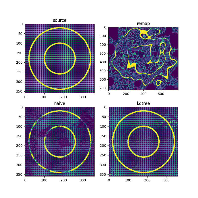
Use KDTree and Inverse Distance Weighting (IDW)

Nibbs

Answer 13

From what I understand you have an original image, and a transformed image, and you wish to recover the nature of the transform that has been applied without knowing it, but assuming it is something sensible, like a rotation or a fish-eye distort.

What I would try is thresholding the image to convert it to binary, in both the index image and the plain image. Then try to identify objects. Most mappings will at least retain connectivity and Euler number, mostly the largest object in the index will still be the largest object in the plain.

Then take moments for your matched image / indexed pairs and see if you can remove translation, rotation and scaling. That gives you several reverse maps, which you can then try to stitch together. (Hard if the transform is not simple, but the general problem of reconstituting just any transformation cannot be solved).

Conwell

No. Given a map M = {X, Y}, I want to compute an inverse map M_inv, such that remap(remap(image_a, M), M_inv) returns image_a, modulo some blanking out of spots that M pushed outside of the frame, loss of resolution due to local stretching, and aliasing due to local condensing. – Holography