Why is the parallel package slower than just using apply?
Asked Answered
S

3

42

I am trying to determine when to use the parallel package to speed up the time necessary to run some analysis. One of the things I need to do is create matrices comparing variables in two data frames with differing number of rows. I asked a question as to an efficient way of doing on StackOverflow and wrote about tests on my blog. Since I am comfortable with the best approach I wanted to speed up the process by running it in parallel. The results below are based upon a 2ghz i7 Mac with 8gb of RAM. I am surprised that the parallel package, the parSapply funciton in particular, is worse than just using the apply function. The code to replicate this is below. Note that I am currently only using one of the two columns I create but eventually want to use both.
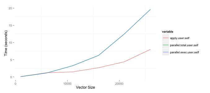
Execution Time
(source: bryer.org)

require(parallel)
require(ggplot2)
require(reshape2)
set.seed(2112)
results <- list()
sizes <- seq(1000, 30000, by=5000)
pb <- txtProgressBar(min=0, max=length(sizes), style=3)
for(cnt in 1:length(sizes)) {
    i <- sizes[cnt]
    df1 <- data.frame(row.names=1:i, 
                      var1=sample(c(TRUE,FALSE), i, replace=TRUE), 
                      var2=sample(1:10, i, replace=TRUE) )
    df2 <- data.frame(row.names=(i + 1):(i + i), 
                      var1=sample(c(TRUE,FALSE), i, replace=TRUE),
                      var2=sample(1:10, i, replace=TRUE))
    tm1 <- system.time({
        df6 <- sapply(df2$var1, FUN=function(x) { x == df1$var1 })
        dimnames(df6) <- list(row.names(df1), row.names(df2))
    })
    rm(df6)
    tm2 <- system.time({
        cl <- makeCluster(getOption('cl.cores', detectCores()))
        tm3 <- system.time({
            df7 <- parSapply(cl, df1$var1, FUN=function(x, df2) { x == df2$var1 }, df2=df2)
            dimnames(df7) <- list(row.names(df1), row.names(df2))
        })
        stopCluster(cl)
    })
    rm(df7)
    results[[cnt]] <- c(apply=tm1, parallel.total=tm2, parallel.exec=tm3)
    setTxtProgressBar(pb, cnt)
}

toplot <- as.data.frame(results)[,c('apply.user.self','parallel.total.user.self',
                          'parallel.exec.user.self')]
toplot$size <- sizes
toplot <- melt(toplot, id='size')

ggplot(toplot, aes(x=size, y=value, colour=variable)) + geom_line() + 
    xlab('Vector Size') + ylab('Time (seconds)')
Sclerodermatous answered 30/1, 2013 at 21:38 Comment(2)
(+1) nice formulation and I find it interesting! (apart from the blog plug :) )Helico
Sorry, didn't mean it as a plug :-) Was just trying to provide all the information I currently have.Sclerodermatous
M
32

Running jobs in parallel incurs overhead. Only if the jobs you fire at the worker nodes take a significant amount of time does parallelization improve overall performance. When the individual jobs take only milliseconds, the overhead of constantly firing off jobs will deteriorate overall performance. The trick is to divide the work over the nodes in such a way that the jobs are sufficiently long, say at least a few seconds. I used this to great effect running six Fortran models simultaneously, but these individual model runs took hours, almost negating the effect of overhead.

Note that I haven't run your example, but the situation I describe above is often the issue when parallization takes longer than running sequentially.

Marseilles answered 30/1, 2013 at 22:3 Comment(2)
Thanks Paul. If you notice I actually track two times, overall which includes the makeCluster call and then one just for my execution so to understand how much overhead there is. From the results it appears there is little overhead in starting the threads. I'm confused as to what overhead there is within the execution.Sclerodermatous
On each of the worker nodes there is an R process, the overhead consists of sending instructions to each node telling them what to do, and gathering back the results.Marseilles
H
23

These differences can be attributed to 1) communication overhead (especially if you run across nodes) and 2) performance overhead (if your job is not that intensive compared to initiating a parallelisation, for example). Usually, if the task you are parallelising is not that time-consuming, then you will mostly find that parallelisation does NOT have much of an effect (which is much highly visible on huge datasets.

Even though this may not directly answer your benchmarking, I hope this should be rather straightforward and can be related to. As an example, here, I construct a data.frame with 1e6 rows with 1e4 unique column group entries and some values in column val. And then I run using plyr in parallel using doMC and without parallelisation.

df <- data.frame(group = as.factor(sample(1:1e4, 1e6, replace = T)), 
                 val = sample(1:10, 1e6, replace = T))
> head(df)
  group val
# 1  8498   8
# 2  5253   6
# 3  1495   1
# 4  7362   9
# 5  2344   6
# 6  5602   9

> dim(df)
# [1] 1000000       2

require(plyr)
require(doMC)
registerDoMC(20) # 20 processors

# parallelisation using doMC + plyr 
P.PLYR <- function() {
    o1 <- ddply(df, .(group), function(x) sum(x$val), .parallel = TRUE)
}

# no parallelisation
PLYR <- function() {
    o2 <- ddply(df, .(group), function(x) sum(x$val), .parallel = FALSE)
}

require(rbenchmark)
benchmark(P.PLYR(), PLYR(), replications = 2, order = "elapsed")

      test replications elapsed relative user.self sys.self user.child sys.child
2   PLYR()            2   8.925    1.000     8.865    0.068      0.000     0.000
1 P.PLYR()            2  30.637    3.433    15.841   13.945      8.944    38.858

As you can see, the parallel version of plyr runs 3.5 times slower

Now, let me use the same data.frame, but instead of computing sum, let me construct a bit more demanding function, say, median(.) * median(rnorm(1e4) ((meaningless, yes):

You'll see that the tides are beginning to shift:

# parallelisation using doMC + plyr 
P.PLYR <- function() {
    o1 <- ddply(df, .(group), function(x) 
      median(x$val) * median(rnorm(1e4)), .parallel = TRUE)
}

# no parallelisation
PLYR <- function() {
    o2 <- ddply(df, .(group), function(x) 
         median(x$val) * median(rnorm(1e4)), .parallel = FALSE)
}

> benchmark(P.PLYR(), PLYR(), replications = 2, order = "elapsed")
      test replications elapsed relative user.self sys.self user.child sys.child
1 P.PLYR()            2  41.911    1.000    15.265   15.369    141.585    34.254
2   PLYR()            2  73.417    1.752    73.372    0.052      0.000     0.000

Here, the parallel version is 1.752 times faster than the non-parallel version.

Edit: Following @Paul's comment, I just implemented a small delay using Sys.sleep(). Of course the results are obvious. But just for the sake of completeness, here's the result on a 20*2 data.frame:

df <- data.frame(group=sample(letters[1:5], 20, replace=T), val=sample(20))

# parallelisation using doMC + plyr 
P.PLYR <- function() {
    o1 <- ddply(df, .(group), function(x) {
    Sys.sleep(2)
    median(x$val)
    }, .parallel = TRUE)
}

# no parallelisation
PLYR <- function() {
    o2 <- ddply(df, .(group), function(x) {
        Sys.sleep(2)
        median(x$val)
    }, .parallel = FALSE)
}

> benchmark(P.PLYR(), PLYR(), replications = 2, order = "elapsed")

#       test replications elapsed relative user.self sys.self user.child sys.child
# 1 P.PLYR()            2   4.116    1.000     0.056    0.056      0.024      0.04
# 2   PLYR()            2  20.050    4.871     0.028    0.000      0.000      0.00

The difference here is not surprising.

Helico answered 30/1, 2013 at 22:6 Comment(3)
+1 for the example code. In the end it all boils down to effectively cutting up your problem in sizeable chunks.Marseilles
A very trivial example is to use a function that just sleeps for ten seconds, there running in parallel really works well. If you cut up a 20 hour job into 60 pieces, parallization is going to present a major improvement. For example processing a satellite image per ten rows of pixels is much efficient than feeding just one pixel per time to the workers, so slice wisely. And in case of plyr, switching to data.table will probably present a much greater improvement than running in parallel. So it is also a matter of choosing the right tool.Marseilles
In addition, when running models in parallel from within R, using six workers presented a 5.6 times increase in performance, but those runs took hours.Marseilles
O
9

Completely agree with @Arun and @PaulHiemestra arguments concerning Why...? part of your question.

However, it seems that you can take some benefits from parallel package in your situation (at least if you are not stuck with Windows). Possible solution is using mclapply instead of parSapply, which relies on fast forking and shared memory.

  tm2 <- system.time({
    tm3 <- system.time({
     df7 <- matrix(unlist(mclapply(df2$var1, FUN=function(x) {x==df1$var1}, mc.cores=8)), nrow=i)
     dimnames(df7) <- list(row.names(df1), row.names(df2))
    })
  })

Of course, nested system.time is not needed here. With my 2 cores I got:

enter image description here

Oney answered 31/1, 2013 at 1:36 Comment(0)

© 2022 - 2024 — McMap. All rights reserved.