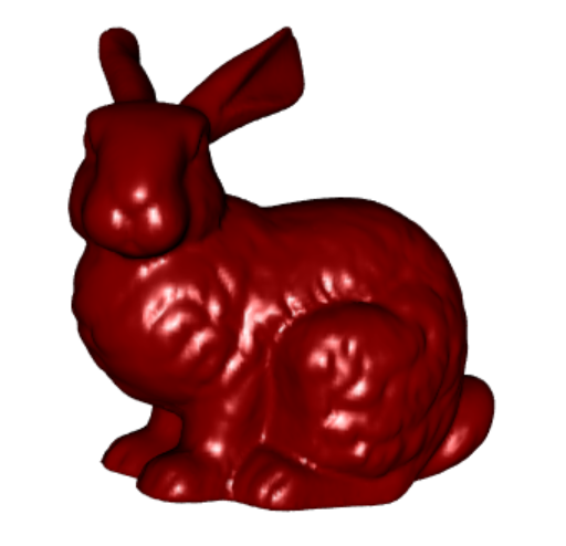
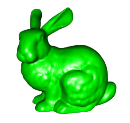
3d surface plot with xyz coordinates

Question

I am hoping someone with experience can help in how one prepares the shape files from xyz data. A great example of a well-prepared dataset can be seen here for the comet Churyumov–Gerasimenko, although the preceding steps in creating the shape file are not provided.

I'm trying to better understand how to apply a surface to a given set of XYZ coordinates. Using Cartesian coordinates is straight forward with the R package "rgl", however shapes that wrap around seem more difficult. I found the R package geometry, which provides an interface to QHULL functions. I tried using this to calculate Delaunay triangulated facets, which I can then plot in rgl. I'm unable to figure out some of the options associated with the function delaunayn to possibly control the maximum distances that these facets are calculated. I am hoping that someone here might have some ideas on improving the surface construction from xyz data.

Example using "Stanford bunnny" dataset:

library(onion)
library(rgl)
library(geometry)
data(bunny)

#XYZ point plot
open3d()
points3d(bunny, col=8, size=0.1)
#rgl.snapshot("3d_bunny_points.png")

#Facets following Delaunay triangulation
tc.bunny <- delaunayn(bunny)
open3d()
tetramesh(tc.bunny, bunny, alpha=0.25, col=8)
#rgl.snapshot("3d_bunny_facets.png")

This answer makes me believe that there might be a problem with the R implementation of Qhull. Also, I have now tried various settings (e.g. delaunayn(bunny, options="Qt")) with little effect. Qhull options are outlined here

Edit:

Here is an additional (simpler) example of a sphere. Even here, the calculation of facets does not always find the closest neighboring vertices (if you rotate the ball you will see some facets crossing through the interior).

library(rgl)
library(geometry)
set.seed(1)
n <- 10
rho <- 1
theta <- seq(0, 2*pi,, n) # azimuthal coordinate running from 0 to 2*pi 
phi <- seq(0, pi,, n) # polar coordinate running from 0 to pi (colatitude)
grd <- expand.grid(theta=theta, phi=phi)

x <- rho * cos(grd$theta) * sin(grd$phi)
y <- rho * sin(grd$theta) * sin(grd$phi)
z <- rho * cos(grd$phi)

set.seed(1)
xyz <- cbind(x,y,z)
tbr = t(surf.tri(xyz, delaunayn(xyz)))
open3d()
rgl.triangles(xyz[tbr,1], xyz[tbr,2], xyz[tbr,3], col = 5, alpha=0.5)
rgl.snapshot("ball.png")

Carmagnole

Have you tried the alphashape3d package? I don't know that it's exactly what you're looking for, but you can get a nicer plot trying this: ashp <- ashape3d(bunny, alpha = c(0.005)); plot(ashp, col=c(8,8,8)) – Morra

@Frank - Thanks for the suggestion, but this example seems to have the same issue - e.g. change alpha = 0.5. – Carmagnole

There's no problem with the R implementation of Qhull in the geometry package: the Delaunay triangulation of a cloud of points is always the same as the Delaunay triangulation of the convex hull of this cloud of points. So your "delaunayised" bunny is convex. – Tiannatiara

Answer 1

Here is an approach using kernel density estimation and the contour3d function from misc3d. I played around until I found a value for levels that worked decently. It's not perfectly precise, but you may be able to tweak things to get a better, more accurate surface. If you have more than 8GB of memory, then you may be able to increase n beyond what I did here.

library(rgl)
library(misc3d)
library(onion); data(bunny)

# the larger the n, the longer it takes, the more RAM you need
bunny.dens <- kde3d(bunny[,1],bunny[,2],bunny[,3], n=150, 
    lims=c(-.1,.2,-.1,.2,-.1,.2)) # I chose lim values manually

contour3d(bunny.dens$d, level = 600, 
    color = "pink", color2 = "green", smooth=500)
rgl.viewpoint(zoom=.75)

The image on the right is from the bottom, just to show another view.

You can use a larger value for n in kde3d but it will take longer, and you may run out of RAM if the array becomes too large. You could also try a different bandwidth (default used here). I took this approach from Computing and Displaying Isosurfaces in R - Feng & Tierney 2008.

---

Very similar isosurface approach using the Rvcg package:

library(Rvcg)
library(rgl)
library(misc3d)
library(onion); data(bunny)

bunny.dens <- kde3d(bunny[,1],bunny[,2],bunny[,3], n=150, 
    lims=c(-.1,.2,-.1,.2,-.1,.2)) # I chose lim values manually

bunny.mesh <- vcgIsosurface(bunny.dens$d, threshold=600)
shade3d(vcgSmooth(bunny.mesh,"HC",iteration=3),col="pink") # do a little smoothing

Since it's a density estimation based approach, we can get a little more out of it by increasing the density of the bunny. I also use n=400 here. The cost is a significant increase in computation time, but the resulting surface is a hare better:

bunny.dens <- kde3d(rep(bunny[,1], 10), # increase density.
                    rep(bunny[,2], 10),
                    rep(bunny[,3], 10), n=400, 
                    lims=c(-.1,.2,-.1,.2,-.1,.2))

bunny.mesh <- vcgIsosurface(bunny.dens$d, threshold=600)
shade3d(vcgSmooth(bunny.mesh,"HC",iteration=1), col="pink")

---

Better, more efficient surface reconstruction methods exist (e.g. power crust, Poisson surface reconstruction, ball-pivot algorithm), but I don't know that any have been implemented in R, yet.

Here's a relevant Stack Overflow post with some great information and links to check out (including links to code): robust algorithm for surface reconstruction from 3D point cloud?.

Morra

Great reference from Feng and Tierney (2008) - just what I've been looking for. I think this will give me a good start into finding related literature on the subject. Thanks for all your help. – Carmagnole

Thanks for your effort here Frank - you brought me a lot further with this topic. I like your rendition of a Silly Putty Bunny! – Carmagnole

Answer 2

I think have found one possible solution using the alphashape3d package. I had to play around a bit to get an acceptable value for alpha, which is related to the distances in the given data set (e.g. sd of bunny gave me some insight). I'm still trying to figure out how to better control the width of lines in vertices and edges so as not to dominate the plot, but this is probably related to settings in rgl.

Example:

library(onion)
library(rgl)
library(geometry)
library(alphashape3d)

data(bunny)
apply(bunny,2,sd)
alphabunny <- ashape3d(bunny, alpha = 0.003)
bg3d(1)
plot.ashape3d(alphabunny, col=c(5,5,5), lwd=0.001, size=0, transparency=rep(0.5,3), indexAlpha = "all")

Edit:

Only by adjusting the plot.ashape3d function, was I able to remove the edges and vertices:

plot.ashape3d.2 <- function (x, clear = TRUE, col = c(2, 2, 2), byComponents = FALSE, 
                             indexAlpha = 1, transparency = 1, walpha = FALSE, ...) 
{
  as3d <- x
  triangles <- as3d$triang
  edges <- as3d$edge
  vertex <- as3d$vertex
  x <- as3d$x
  if (class(indexAlpha) == "character") 
    if (indexAlpha == "ALL" | indexAlpha == "all") 
      indexAlpha = 1:length(as3d$alpha)
  if (any(indexAlpha > length(as3d$alpha)) | any(indexAlpha <= 
                                                   0)) {
    if (max(indexAlpha) > length(as3d$alpha)) 
      error = max(indexAlpha)
    else error = min(indexAlpha)
    stop(paste("indexAlpha out of bound : valid range = 1:", 
               length(as3d$alpha), ", problematic value = ", error, 
               sep = ""), call. = TRUE)
  }
  if (clear) {
    rgl.clear()
  }
  if (byComponents) {
    components = components_ashape3d(as3d, indexAlpha)
    if (length(indexAlpha) == 1) 
      components = list(components)
    indexComponents = 0
    for (iAlpha in indexAlpha) {
      if (iAlpha != indexAlpha[1]) 
        rgl.open()
      if (walpha) 
        title3d(main = paste("alpha =", as3d$alpha[iAlpha]))
      cat("Device ", rgl.cur(), " : alpha = ", as3d$alpha[iAlpha], 
          "\n")
      indexComponents = indexComponents + 1
      components[[indexComponents]][components[[indexComponents]] == 
                                      -1] = 0
      colors = c("#000000", sample(rainbow(max(components[[indexComponents]]))))
      tr <- t(triangles[triangles[, 8 + iAlpha] == 2 | 
                          triangles[, 8 + iAlpha] == 3, c("tr1", "tr2", 
                                                          "tr3")])
      if (length(tr) != 0) 
        rgl.triangles(x[tr, 1], x[tr, 2], x[tr, 3], col = colors[1 + 
                                                                   components[[indexComponents]][tr]], alpha = transparency, 
                      ...)
    }
  }
  else {
    for (iAlpha in indexAlpha) {
      if (iAlpha != indexAlpha[1]) 
        rgl.open()
      if (walpha) 
        title3d(main = paste("alpha =", as3d$alpha[iAlpha]))
      cat("Device ", rgl.cur(), " : alpha = ", as3d$alpha[iAlpha], 
          "\n")
      tr <- t(triangles[triangles[, 8 + iAlpha] == 2 | 
                          triangles[, 8 + iAlpha] == 3, c("tr1", "tr2", 
                                                          "tr3")])
      if (length(tr) != 0) 
        rgl.triangles(x[tr, 1], x[tr, 2], x[tr, 3], col = col[1], 
                      , alpha = transparency, ...)
    }
  }
}

alphabunny <- ashape3d(bunny, alpha = c(0.003))
plot.ashape3d.2(alphabunny, col=5, indexAlpha = "all", transparency=1)
bg3d(1)

Carmagnole

So, my answer did work for you! I didn't post it as an answer because I wasn't sure it was what you needed. Anyway, you only need to use indexAlpha = "all" if you used more than one alpha value in your call to ashape3d and you want to plot the results for all the alpha values you tried. – Morra

@Frank - I honestly didn't realize that this was the same package that you recommended! I came across it through another Google search and the package's vignette helped me figure the settings out. I'll try your recommendations out. Cheers! – Carmagnole

@Frank - Looks like I confused alpha with transparency. You should write a formal answer here. – Carmagnole

That second plot with your adjusted plot.ashape3d.2 is pretty cool! I found that alpha = 0.0015 makes for a pretty nice image. – Morra

@Frank - Yes, alpha = 0.0015 gives a better result in some places, but there's holes all over if you look closely. – Carmagnole

Answer 3

The package Rvcg updated to version 0.14 in July 2016, and ball pivoting surface reconstruction was added. The function is vcgBallPivoting:

library(Rvcg) # needs to be >= version 0.14
library(rgl)
library(onion); data(bunny)

# default parameters
bunnybp <- vcgBallPivoting(bunny, radius = 0.0022, clustering = 0.2, angle = pi/2)
shade3d(bunnybp, col = rainbow(1000), specular = "black")
shade3d(bunnybp, col = "pink", specular = "black") # easier to see problem areas.

The ball pivoting and the default parameter settings are not perfect for the Stanford bunny (as noted by cuttlefish44 in the comments radius = 0.0022 does better than the default radius = 0), and you are left with some gaps in the surface. The actual bunny has 2 holes in the base and some scanning limitations contribute to a few other holes (as mentioned here: https://graphics.stanford.edu/software/scanview/models/bunny.html). You may be able to find better parameters, and it's quite fast to use vcgBallPivoting (~0.5 seconds on my machine), but additional effort / methods may be required to close the gaps.

Morra

This is really fast - thanks for the answer. Unfortunately, I haven't been able to get rid of those holes by playing around with the argument parameters. BTW, the vcgBallPivoting function crashes R when using RStudio. I've notified the package authors. – Carmagnole

Your answer is so interesting for me. radius = 0.0022 returns better output, but not perfect... – Jenjena

Answer 4

I'm currently making a package, RCGAL, which currently offers two types of surface reconstruction. It is based on the RcppCGAL package, which links to the header files of the C++ library CGAL (Computational Geometry Algorithms Library).

Here is the advanced front surface reconstruction of the Stanford bunny:

Here is the Poisson surface reconstruction of the Stanford bunny with the default parameters:

This mesh is not very precise. One gets a more precise mesh by using a smaller value of the spacing parameter:

See this blog post for more info.

Hoban

This looks very nice. Perhaps you should provide code for your answer so that others may reproduce. – Carmagnole

@Marcinthebox added link to my blog – Tiannatiara