How to calculate the regularization parameter in linear regression

Question

When we have a high degree linear polynomial that is used to fit a set of points in a linear regression setup, to prevent overfitting, we use regularization, and we include a lambda parameter in the cost function. This lambda is then used to update the theta parameters in the gradient descent algorithm.

My question is how do we calculate this lambda regularization parameter?

Entomophagous

Answer 1

The regularization parameter (lambda) is an input to your model so what you probably want to know is how do you select the value of lambda. The regularization parameter reduces overfitting, which reduces the variance of your estimated regression parameters; however, it does this at the expense of adding bias to your estimate. Increasing lambda results in less overfitting but also greater bias. So the real question is "How much bias are you willing to tolerate in your estimate?"

One approach you can take is to randomly subsample your data a number of times and look at the variation in your estimate. Then repeat the process for a slightly larger value of lambda to see how it affects the variability of your estimate. Keep in mind that whatever value of lambda you decide is appropriate for your subsampled data, you can likely use a smaller value to achieve comparable regularization on the full data set.

Libertarian

Does adding a regularization parameter reduce the variance of the parameters? does that mean they all will be almost equal in magnitude? Is that the variance in their values you refer to? – Entomophagous

Yes, it reduces the variance of the parameters. Let's assume that you have K parameters (a_1,a_2,...,a_K) in your linear model and your sample size is N. Given a particular sample of size N, you will compute the values a_1 through a_k. If you were to take another random sample of size N, it would result in a different set of coefficients (a). If your sample size is small, then a particular coefficient (e.g., a_1) can vary greatly between samples (high variance). Regularization reduces this variance. It doesn't mean that all the coefficients (a_1 ... a_k) will be nearly equal. – Libertarian

Answer 2

CLOSED FORM (TIKHONOV) VERSUS GRADIENT DESCENT

Hi! nice explanations for the intuitive and top-notch mathematical approaches there. I just wanted to add some specificities that, where not "problem-solving", may definitely help to speed up and give some consistency to the process of finding a good regularization hyperparameter.

I assume that you are talking about the L2 (a.k. "weight decay") regularization, linearly weighted by the lambda term, and that you are optimizing the weights of your model either with the closed-form Tikhonov equation (highly recommended for low-dimensional linear regression models), or with some variant of gradient descent with backpropagation. And that in this context, you want to choose the value for lambda that provides best generalization ability.

---

CLOSED FORM (TIKHONOV)

If you are able to go the Tikhonov way with your model (Andrew Ng says under 10k dimensions, but this suggestion is at least 5 years old) Wikipedia - determination of the Tikhonov factor offers an interesting closed-form solution, which has been proven to provide the optimal value. But this solution probably raises some kind of implementation issues (time complexity/numerical stability) I'm not aware of, because there is no mainstream algorithm to perform it. This 2016 paper looks very promising though and may be worth a try if you really have to optimize your linear model to its best.

• For a quicker prototype implementation, this 2015 Python package seems to deal with it iteratively, you could let it optimize and then extract the final value for the lambda:

In this new innovative method, we have derived an iterative approach to solving the general Tikhonov regularization problem, which converges to the noiseless solution, does not depend strongly on the choice of lambda, and yet still avoids the inversion problem.

And from the GitHub README of the project: InverseProblem.invert(A, be, k, l) #this will invert your A matrix, where be is noisy be, k is the no. of iterations, and lambda is your dampening effect (best set to 1)

---

GRADIENT DESCENT

All links of this part are from Michael Nielsen's amazing online book "Neural Networks and Deep Learning", recommended reading!

For this approach it seems to be even less to be said: the cost function is usually non-convex, the optimization is performed numerically and the performance of the model is measured by some form of cross validation (see Overfitting and Regularization and why does regularization help reduce overfitting if you haven't had enough of that). But even when cross-validating, Nielsen suggests something: you may want to take a look at this detailed explanation on how does the L2 regularization provide a weight decaying effect, but the summary is that it is inversely proportional to the number of samples n, so when calculating the gradient descent equation with the L2 term,

just use backpropagation, as usual, and then add (λ/n)*w to the partial derivative of all the weight terms.

And his conclusion is that, when wanting a similar regularization effect with a different number of samples, lambda has to be changed proportionally:

we need to modify the regularization parameter. The reason is because the size n of the training set has changed from n=1000 to n=50000, and this changes the weight decay factor 1−learning_rate*(λ/n). If we continued to use λ=0.1 that would mean much less weight decay, and thus much less of a regularization effect. We compensate by changing to λ=5.0.

This is only useful when applying the same model to different amounts of the same data, but I think it opens up the door for some intuition on how it should work, and, more importantly, speed up the hyperparametrization process by allowing you to finetune lambda in smaller subsets and then scale up.

For choosing the exact values, he suggests in his conclusions on how to choose a neural network's hyperparameters the purely empirical approach: start with 1 and then progressively multiply&divide by 10 until you find the proper order of magnitude, and then do a local search within that region. In the comments of this SE related question, the user Brian Borchers suggests also a very well known method that may be useful for that local search:

1. Take small subsets of the training and validation sets (to be able to make many of them in a reasonable amount of time)
2. Starting with λ=0 and increasing by small amounts within some region, perform a quick training&validation of the model and plot both loss functions
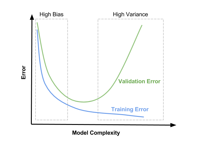
3. You will observe three things:
   • The CV loss function will be consistently higher than the training one, since your model is optimized for the training data exclusively (EDIT: After some time I've seen a MNIST case where adding L2 helped the CV loss decrease faster than the training one until convergence. Probably due to the ridiculous consistency of the data and a suboptimal hyperparametrization though).
   • The training loss function will have its minimum for λ=0, and then increase with the regularization, since preventing the model from optimally fitting the training data is exactly what regularization does.
   • The CV loss function will start high at λ=0, then decrease, and then start increasing again at some point (EDIT: this assuming that the setup is able to overfit for λ=0, i.e. the model has enough power and no other regularization means are heavily applied).
4. The optimal value for λ will be probably somewhere around the minimum of the CV loss function, it also may depend a little on how does the training loss function look like. See the picture for a possible (but not the only one) representation of this: instead of "model complexity" you should interpret the x axis as λ being zero at the right and increasing towards the left.

Hope this helps! Cheers,
Andres

Sough

Answer 3

The cross validation described above is a method used often in Machine Learning. However, choosing a reliable and safe regularization parameter is still a very hot topic of research in mathematics. If you need some ideas (and have access to a decent university library) you can have a look at this paper: http://www.sciencedirect.com/science/article/pii/S0378475411000607

Folk

And if you don't have access to a decent university library, it seems to be available here. – Darcidarcia

@Darcidarcia Thank you for liberating knowledge and education. Ha, the websites URL of the post ... Should rather be called ScienceIndirect. – Altdorfer

Answer 4

use Cross-validation from sklearn library and its sklearn.linear_model.RidgeCV or sklearn.linear_model.LassoCV. Its method score(X, y[, sample_weight]) returns the R2 coefficient of determination of the prediction (showing how well the data fit the regression model, though " low R² doesn't guarantee a bad fit, and a high R² doesn't guarantee a good fit!"). Best possible score is 1.0, lower values are worse. - so the bigger - the better, choose the best. Or can choose best_score automatically when doing Cross-Validation with GridSearchCV. Better try multi-metric evaluation

P.S. I would also advise to pay attention to these criteria (as for model selection) - Linear regression - Model selection criteria - Which criterion to use, Model selection criteria, Choice of a regularization parameter, rank-deficiency and Condition Number and Handling Multicollinear Features

P.P.S. Regularization of covariance matrix, 6.2 Regularizing a Correlation Matrix AND 2.1 Variable Selection - for good Regression model - remove Outliers, remove Multicollinearity (for OLS to be BLUE - What it means to be best), be careful with p-value, that shows statistical significance, as it can be significant under the certain circumstances or in certain sample, - to avoid this - use t-test & F-test on different samples...- this matters for Inferential Statistics. However, for Predictive Statistics multicollinearity cannot harm. Nevertheless, knowledge of experimental design are always valuable

P.P.P.S. mathematically Closed-form solution of Ridge

Cassiopeia