Code for best fit straight line of a scatter plot

Question

Below is my code for scatter plotting the data in my text file. The file I am opening contains two columns. The left column is x coordinates and the right column is y coordinates. the code creates a scatter plot of x vs. y. I need a code to overplot a line of best fit to the data in the scatter plot, and none of the built in pylab function have worked for me.

from matplotlib import *
from pylab import *

with open('file.txt') as f:
   data = [line.split() for line in f.readlines()]
   out = [(float(x), float(y)) for x, y in data]
for i in out:
   scatter(i[0],i[1])
   xlabel('X')
   ylabel('Y')
   title('My Title')
show()

Showers

possible duplicate of fitting a curved best fit line to a data set in python – Fowling

I don't need a curved best fit line, I need a straight best fit line – Showers

dg99, I've looked at that link prior to creating this question and I tried techniques from the link with no success. – Showers

Can you show us the code that you tried with the polyfit function and describe how it didn't work? Remember to set the deg parameter to 1 in order to get a linear fit. (See docs here.) – Fowling

Answer 1

A one-line version of this excellent answer to plot the line of best fit is:

plt.plot(np.unique(x), np.poly1d(np.polyfit(x, y, 1))(np.unique(x)))

Using np.unique(x) instead of x handles the case where x isn't sorted or has duplicate values.

Lathing

I don't understand the (x) at the end. I checked the scipy documentation and don't see an explanation there. How did you know to use that syntax with poly1d? – Townsville

@Townsville poly1d returns a function for the line of best fit, which you then evaluate at the points x. – Indistinguishable

Is there a way to extend the best fit line beyond the original x axis? – Amedeo

@FortuneFaded: Yes, replace the second np.unique(x) with a 1D array of the x points you'd like to plot the line at. – Indistinguishable

^ Whoops, you have to replace both of the np.unique(x), not just the second one like I said above. – Indistinguishable

Maybe you can explain this code out? I'm a bit confused what np.ploy1d and how it workks with the rest of the code. thanks – Lepidopterous

@Lepidopterous in this case, it's basically equivalent to converting the slope and intercept returned by polyfit (np.array([m, b])) into a function lambda x: m * x + b which you can then evaluate at the points np.unique(x). – Indistinguishable

in my case where I had only y I used the following code: plt.plot(range(y), np.poly1d(np.polyfit(range(y), y, 1))(np.unique(range(y)))) – Corroborant

Answer 2

Assuming line of best fit for a set of points is:

y = a + b * x

where:

b = ( sum(xi * yi) - n * xbar * ybar ) / sum((xi - xbar)^2)
a = ybar - b * xbar

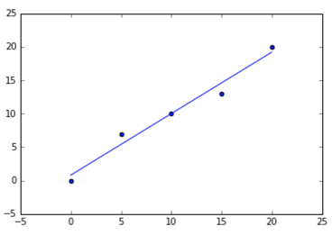
Code and plot

# sample points 
X = [0, 5, 10, 15, 20]
Y = [0, 7, 10, 13, 20]

# solve for a and b
def best_fit(X, Y):

    xbar = sum(X)/len(X)
    ybar = sum(Y)/len(Y)
    n = len(X) # or len(Y)

    numer = sum([xi*yi for xi,yi in zip(X, Y)]) - n * xbar * ybar
    denum = sum([xi**2 for xi in X]) - n * xbar**2

    b = numer / denum
    a = ybar - b * xbar

    print('best fit line:\ny = {:.2f} + {:.2f}x'.format(a, b))

    return a, b

# solution
a, b = best_fit(X, Y)
#best fit line:
#y = 0.80 + 0.92x

# plot points and fit line
import matplotlib.pyplot as plt
plt.scatter(X, Y)
yfit = [a + b * xi for xi in X]
plt.plot(X, yfit)

UPDATE:

notebook version

Ohl

Exactly what I was looking for. Useful that the matplot lib isn't mixed in with the actual LOB algorithm. Thank you Aziz. – Underproof

I had to convert numer and denum to floats. Otherwise I get the wrong result. – Bridgeport

numer = float(sum([xi*yi for xi,yi in zip(X, Y)]) - n * xbar * ybar) denum = float(sum([xi2 for xi in X]) - n * xbar2) – Bridgeport

@AzizAlto Great work!!. Just want to know how to find the end (x,y) coordinates of this best fit line ? – Keeler

@ShubhamS.Naik thanks, do you mean the last X and yfit points? if so they would, X[-1] and yfit[-1] – Ohl

Works in Python 2.7 if you change the sample data points to floats, X = [0.0, 5.0, 10.0, 15.0, 20.0] Y = [0.0, 7.0, 10.0, 13.0, 20.0] – Contrariety

I've done a little testing and this algorithm is about 5x faster than sklearn.linear_model.LinearRegression – Cirone

Answer 3

You can use numpy's polyfit. I use the following (you can safely remove the bit about coefficient of determination and error bounds, I just think it looks nice):

#!/usr/bin/python3

import numpy as np
import matplotlib.pyplot as plt
import csv

with open("example.csv", "r") as f:
    data = [row for row in csv.reader(f)]
    xd = [float(row[0]) for row in data]
    yd = [float(row[1]) for row in data]

# sort the data
reorder = sorted(range(len(xd)), key = lambda ii: xd[ii])
xd = [xd[ii] for ii in reorder]
yd = [yd[ii] for ii in reorder]

# make the scatter plot
plt.scatter(xd, yd, s=30, alpha=0.15, marker='o')

# determine best fit line
par = np.polyfit(xd, yd, 1, full=True)

slope=par[0][0]
intercept=par[0][1]
xl = [min(xd), max(xd)]
yl = [slope*xx + intercept  for xx in xl]

# coefficient of determination, plot text
variance = np.var(yd)
residuals = np.var([(slope*xx + intercept - yy)  for xx,yy in zip(xd,yd)])
Rsqr = np.round(1-residuals/variance, decimals=2)
plt.text(.9*max(xd)+.1*min(xd),.9*max(yd)+.1*min(yd),'$R^2 = %0.2f$'% Rsqr, fontsize=30)

plt.xlabel("X Description")
plt.ylabel("Y Description")

# error bounds
yerr = [abs(slope*xx + intercept - yy)  for xx,yy in zip(xd,yd)]
par = np.polyfit(xd, yerr, 2, full=True)

yerrUpper = [(xx*slope+intercept)+(par[0][0]*xx**2 + par[0][1]*xx + par[0][2]) for xx,yy in zip(xd,yd)]
yerrLower = [(xx*slope+intercept)-(par[0][0]*xx**2 + par[0][1]*xx + par[0][2]) for xx,yy in zip(xd,yd)]

plt.plot(xl, yl, '-r')
plt.plot(xd, yerrLower, '--r')
plt.plot(xd, yerrUpper, '--r')
plt.show()

Gayla

Answer 4

Have implemented @Micah 's solution to generate a trendline with a few changes and thought I'd share:

• Coded as a function
• Option for a polynomial trendline (input order=2)
• Function can also just return the coefficient of determination (R^2, input Rval=True)
• More Numpy array optimisations

Code:

def trendline(xd, yd, order=1, c='r', alpha=1, Rval=False):
    """Make a line of best fit"""

    #Calculate trendline
    coeffs = np.polyfit(xd, yd, order)

    intercept = coeffs[-1]
    slope = coeffs[-2]
    power = coeffs[0] if order == 2 else 0

    minxd = np.min(xd)
    maxxd = np.max(xd)

    xl = np.array([minxd, maxxd])
    yl = power * xl ** 2 + slope * xl + intercept

    #Plot trendline
    plt.plot(xl, yl, c, alpha=alpha)

    #Calculate R Squared
    p = np.poly1d(coeffs)

    ybar = np.sum(yd) / len(yd)
    ssreg = np.sum((p(xd) - ybar) ** 2)
    sstot = np.sum((yd - ybar) ** 2)
    Rsqr = ssreg / sstot

    if not Rval:
        #Plot R^2 value
        plt.text(0.8 * maxxd + 0.2 * minxd, 0.8 * np.max(yd) + 0.2 * np.min(yd),
                 '$R^2 = %0.2f$' % Rsqr)
    else:
        #Return the R^2 value:
        return Rsqr

Kaleb

Answer 5

import matplotlib.pyplot as plt    
from sklearn.linear_model import LinearRegression

X, Y = x.reshape(-1,1), y.reshape(-1,1)
plt.plot( X, LinearRegression().fit(X, Y).predict(X) )

Vereen

Answer 6

Numpy 1.4 introduced new API. You can use this one-liner, where n determines how smooth you want the line to be and a is the degree of the polynomial.

plt.plot(*np.polynomial.Polynomial.fit(x, y, a).linspace(n), 'r-')

Downwind