Inserting an image to ggplot2
Asked Answered
Z

4

73

Is it possible to insert a raster image or a pdf image underneath a geom_line() on a ggplot2 plot?

I wanted to be quickly able to plot data over a previously calculated plot that takes a long time to generate as it uses a large amount of data.

I read through this example. However, as it is over one year old I thought there might be a different way of doing this now.

Zymometer answered 28/3, 2012 at 23:18 Comment(0)
E
102

try ?annotation_custom in ggplot2

example,

library(png)
library(grid)
img <- readPNG(system.file("img", "Rlogo.png", package="png"))
g <- rasterGrob(img, interpolate=TRUE)

qplot(1:10, 1:10, geom="blank") +
  annotation_custom(g, xmin=-Inf, xmax=Inf, ymin=-Inf, ymax=Inf) +
  geom_point()
Elaterid answered 29/3, 2012 at 0:40 Comment(6)
Is it possible to read in an external file such as a .jpg or .pdf to use with `annotation_custom()' ? I read through some examples but the annotation seems to be generated in R.Zymometer
i added an example for a bitmap. With a vector image, you'll need to create a grob with the grImport package.Elaterid
This doesn't seem to work if wanting to add two of the same image. How would one do this?Cosmism
@Cosmism for a reason I don't understand, the grobs need to have unique names. Try g2 = editGrob(g, name="newgrob")Elaterid
Note that this does not work with coord_polar, but one can find a solution for that case at this question #34496500.Homegrown
When I save the result image from above with ggsave(filename="plotwithr.png"), load it again with img <- readPNG("plotwithr.png") and then do the qplot again with this grob, why does it not cover the entire area and shrinks instead?Trost
J
56

Could also use the cowplot R package (cowplot is a powerful extension of ggplot2). It will also need the magick package. Check this introduction to cowplot vignette.

Here is an example for both PNG and PDF background images.

library(ggplot2)
library(cowplot)
library(magick)

# Update 2020-04-15: 
# As of version 1.0.0, cowplot does not change the default ggplot2 theme anymore.
# So, either we add theme_cowplot() when we build the graph 
# (commented out in the example below), 
# or we set theme_set(theme_cowplot()) at the beginning of our script:
theme_set(theme_cowplot())

my_plot <- 
  ggplot(data    = iris, 
         mapping = aes(x    = Sepal.Length, 
                       fill = Species)) + 
  geom_density(alpha = 0.7) # +
  # theme_cowplot()

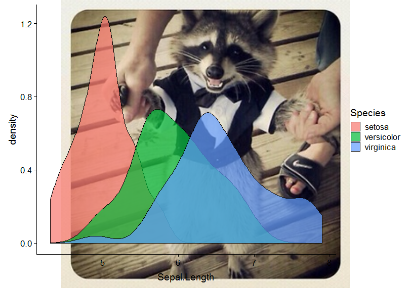
# Example with PNG (for fun, the OP's avatar - I love the raccoon)
ggdraw() +
  draw_image("https://i.sstatic.net/WDOo4.jpg?s=328&g=1") +
  draw_plot(my_plot)

enter image description here

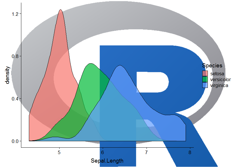
# Example with PDF
ggdraw() +
  draw_image(file.path(R.home(), "doc", "html", "Rlogo.pdf")) +
  draw_plot(my_plot)

enter image description here

Also, as @seabass20 asked in the comment below, we can also give a custom position and scale to the image. Below is an example inspired from help(draw_image). One needs to fine tune the parameters x, y, and scale until gets the desired output.

logo_file <- system.file("extdata", "logo.png", package = "cowplot")
my_plot_2 <- ggdraw() +
  draw_image(logo_file,  x = 0.3, y = 0.4, scale = .2) +
  draw_plot(my_plot)
my_plot_2

Created on 2020-04-15 by the reprex package (v0.3.0)

Jilleen answered 16/10, 2018 at 19:50 Comment(2)
Is it possible to specify where the image should go (i.e. if I want the image just in the top-right corner of my plot)? Thanks!Celerity
@seabass20, Thanks for your comment. I made an extra example in my answer to accommodate your needs. You can always find more examples and details in help(draw_image). Hope it helped.Important
J
27

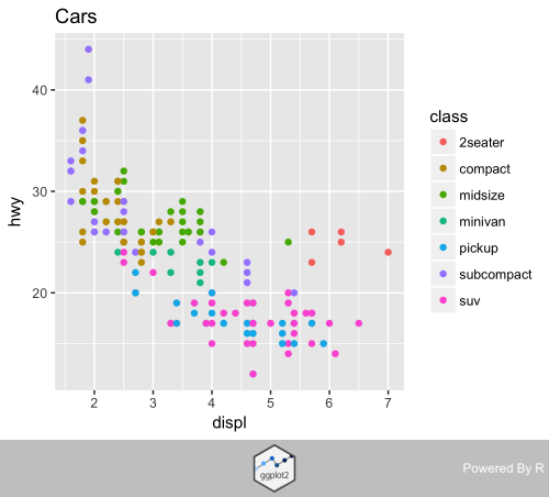
Just adding an update from the terrific Magick package:

library(ggplot2)
library(magick)
library(here) # For making the script run without a wd
library(magrittr) # For piping the logo

# Make a simple plot and save it
ggplot(mpg, aes(displ, hwy, colour = class)) + 
  geom_point() + 
  ggtitle("Cars") +
  ggsave(filename = paste0(here("/"), last_plot()$labels$title, ".png"),
         width = 5, height = 4, dpi = 300)

# Call back the plot
plot <- image_read(paste0(here("/"), "Cars.png"))
# And bring in a logo
logo_raw <- image_read("http://hexb.in/hexagons/ggplot2.png") 

# Scale down the logo and give it a border and annotation
# This is the cool part because you can do a lot to the image/logo before adding it
logo <- logo_raw %>%
  image_scale("100") %>% 
  image_background("grey", flatten = TRUE) %>%
  image_border("grey", "600x10") %>%
  image_annotate("Powered By R", color = "white", size = 30, 
                 location = "+10+50", gravity = "northeast")

# Stack them on top of each other
final_plot <- image_append(image_scale(c(plot, logo), "500"), stack = TRUE)
# And overwrite the plot without a logo
image_write(final_plot, paste0(here("/"), last_plot()$labels$title, ".png"))

Cars with logo

Jigger answered 11/7, 2017 at 23:11 Comment(0)
S
5

Following up on @baptiste's answer, you don't need to load the grob package and convert the image if you use the more specific annotation function annotation_raster().

That quicker option could look like this:

# read picture
library(png)
img <- readPNG(system.file("img", "Rlogo.png", package = "png"))
# plot with picture as layer
library(ggplot2)
ggplot(mapping = aes(1:10, 1:10)) +
  annotation_raster(img, xmin = -Inf, xmax = Inf, ymin = -Inf, ymax = Inf) +
  geom_point()

Created on 2021-02-16 by the reprex package (v1.0.0)

Sarena answered 16/2, 2021 at 7:17 Comment(2)
But you can't change the size of image in this way.Glanville
You can change the size of the image by changing the values in xmin, xmax, ymin, ymaxConfounded

© 2022 - 2024 — McMap. All rights reserved.