What does the parameter retain_graph mean in the Variable's backward() method?

Question

I'm going through the neural transfer pytorch tutorial and am confused about the use of retain_variable(deprecated, now referred to as retain_graph). The code example show:

class ContentLoss(nn.Module):

    def __init__(self, target, weight):
        super(ContentLoss, self).__init__()
        self.target = target.detach() * weight
        self.weight = weight
        self.criterion = nn.MSELoss()

    def forward(self, input):
        self.loss = self.criterion(input * self.weight, self.target)
        self.output = input
        return self.output

    def backward(self, retain_variables=True):
        #Why is retain_variables True??
        self.loss.backward(retain_variables=retain_variables)
        return self.loss

From the documentation

retain_graph (bool, optional) – If False, the graph used to compute the grad will be freed. Note that in nearly all cases setting this option to True is not needed and often can be worked around in a much more efficient way. Defaults to the value of create_graph.

So by setting retain_graph= True, we're not freeing the memory allocated for the graph on the backward pass. What is the advantage of keeping this memory around, why do we need it?

Maddening

Answer 1

@cleros is pretty on the point about the use of retain_graph=True. In essence, it will retain any necessary information to calculate a certain variable, so that we can do backward pass on it.

An illustrative example

Suppose that we have a computation graph shown above. The variable d and e is the output, and a is the input. For example,

import torch
from torch.autograd import Variable
a = Variable(torch.rand(1, 4), requires_grad=True)
b = a**2
c = b*2
d = c.mean()
e = c.sum()

when we do d.backward(), that is fine. After this computation, the parts of the graph that calculate d will be freed by default to save memory. So if we do e.backward(), the error message will pop up. In order to do e.backward(), we have to set the parameter retain_graph to True in d.backward(), i.e.,

d.backward(retain_graph=True)

As long as you use retain_graph=True in your backward method, you can do backward any time you want:

d.backward(retain_graph=True) # fine
e.backward(retain_graph=True) # fine
d.backward() # also fine
e.backward() # error will occur!

More useful discussion can be found here.

A real use case

Right now, a real use case is multi-task learning where you have multiple losses that maybe be at different layers. Suppose that you have 2 losses: loss1 and loss2 and they reside in different layers. In order to backprop the gradient of loss1 and loss2 w.r.t to the learnable weight of your network independently. You have to use retain_graph=True in backward() method in the first back-propagated loss.

# suppose you first back-propagate loss1, then loss2 (you can also do the reverse)
loss1.backward(retain_graph=True)
loss2.backward() # now the graph is freed, and next process of batch gradient descent is ready

optimizer.step() # update the network parameters

Tavis

To avoid having to use retain_graph=True you could just do loss = loss1 + loss2 then loss.backward() – Bacolod

@BrandonBrown Are the two methods mathematically equivalent? – Underlay

@PrzemekD I think it is equivalent as long as you do not use coefficients when adding them together. – Tavis

That's true, but it's important to remember that that condition is violated if you're using adaptive gradient methods like ADAM. – Mayers

@SamBobel can you please provide a bit more information about that? As I am adding two losses at two different layers and optimizing them using ADAM. How is it different from optimizing both losses independently? – Alp

@MAsadAli I'll try. Each copy of ADAM stores adaptive learning rate parameters, which represent how "smooth" the loss function is in parameter-space. If the two losses are different smoothnesses, it may have trouble picking a value that works for both. (1/2) – Mayers

Let's say loss 1 varies rapidly with your parameters, but is small in magnitude. You'd need small steps to optimize it, because it's not smooth. And loss 2 varies slowly, but is big in magnitude. #2 will dominate their sum, so one shared ADAM will choose a big learning rate. But if you keep them separate, ADAM will chose a big learning rate for loss #2 and a small learning rate for loss #1. (2/2) – Mayers

@SamBobel Does that mean the optimization path of dividing and combining the two losses could be different? I mean it seems your statement indicates dealing with the losses in a separately could be more efficient? – Notional

They are definitely different. "Efficient" is tough -- You clearly use less parameters if you combine them, and it's faster computationally as well. Which works better in practice for your problem is 100% an empirical question. Hopefully my last example is clear enough to explain the different behaviors. – Mayers

if change the order of code to:a = Variable(torch.rand(1, 4), requires_grad=True) b = a**2 c = b*2 d = c.mean() d.backward() e = c.sum() e.backward(), that is to say move e=c.sum() after d.backward(), why pytorch would not rebuild a new computational graph for e ? – Rhyton

Answer 2

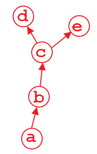
This is a very useful feature when you have more than one output of a network. Here's a completely made up example: imagine you want to build some random convolutional network that you can ask two questions of: Does the input image contain a cat, and does the image contain a car?

One way of doing this is to have a network that shares the convolutional layers, but that has two parallel classification layers following (forgive my terrible ASCII graph, but this is supposed to be three convlayers, followed by three fully connected layers, one for cats and one for cars):

                    -- FC - FC - FC - cat?
Conv - Conv - Conv -|
                    -- FC - FC - FC - car?

Given a picture that we want to run both branches on, when training the network, we can do so in several ways. First (which would probably be the best thing here, illustrating how bad the example is), we simply compute a loss on both assessments and sum the loss, and then backpropagate.

However, there's another scenario - in which we want to do this sequentially. First we want to backprop through one branch, and then through the other (I have had this use-case before, so it is not completely made up). In that case, running .backward() on one graph will destroy any gradient information in the convolutional layers, too, and the second branch's convolutional computations (since these are the only ones shared with the other branch) will not contain a graph anymore! That means, that when we try to backprop through the second branch, Pytorch will throw an error since it cannot find a graph connecting the input to the output! In these cases, we can solve the problem by simple retaining the graph on the first backward pass. The graph will then not be consumed, but only be consumed by the first backward pass that does not require to retain it.

EDIT: If you retain the graph at all backward passes, the implicit graph definitions attached to the output variables will never be freed. There might be a usecase here as well, but I cannot think of one. So in general, you should make sure that the last backwards pass frees the memory by not retaining the graph information.

As for what happens for multiple backward passes: As you guessed, pytorch accumulates gradients by adding them in-place (to a variable's/parameters .grad property). This can be very useful, since it means that looping over a batch and processing it once at a time, accumulating the gradients at the end, will do the same optimization step as doing a full batched update (which only sums up all the gradients as well). While a fully batched update can be parallelized more, and is thus generally preferable, there are cases where batched computation is either very, very difficult to implement or simply not possible. Using this accumulation, however, we can still rely on some of the nice stabilizing properties that batching brings. (If not on the performance gain)

Gillespie

Thanks, that's super helpful! A couple of follow up questions: 1. What happens if all of your backward passes retain the graph? Is this just a waste of memory or will other issues come up? 2. In your example, say we're also training all of the convolutional layers. On the first backward pass, their gradients will be computed for each layer. When we run the second backward pass, are the gradients for the same convolutional layer added together? – Maddening

Added an answer to your comment to the answer :-) – Gillespie

That mostly makes sense to me. It still seems like even if you run backward with retain_graph=False on your last backward pass, the branch that isn't shared e.g. the one that ran first, still won't have it's resources cleared up. In your example, Conv -> Conv -> Conv get's freed in the shared branch but not -- FC - FC - FC - cat? – Maddening