Seeking workaround for gtable_add_grob code broken by ggplot 2.2.0
Asked Answered
M

2

17

In plots with multiple facet variables, ggplot2 repeats the facet label for the "outer" variable, rather than having a single spanning facet strip across all the levels of the "inner" variable. I have some code that I've been using to cover the repeated outer facet labels with a single spanning facet strip using gtable_add_grob from the gtable package.

Unfortunately, this code no longer works with ggplot2 2.2.0 due to changes in the grob structure of the facet strips. Specifically, in previous versions of ggplot2, each row of facet labels got their own set of grobs. However, in version 2.2.0 it looks like each vertical stack of facet labels is a single grob. This breaks my code and I'm not sure how to fix it.

Here's a concrete example, taken from an SO question I answered a few months ago:

# Data
df = structure(list(location = structure(c(1L, 1L, 1L, 1L, 1L, 1L, 
    1L, 1L, 1L, 1L, 2L, 2L, 2L, 2L, 2L, 2L, 2L, 2L, 2L, 2L, 1L, 1L, 
    1L, 1L, 1L, 1L, 1L, 1L, 1L, 1L, 2L, 2L, 2L, 2L, 2L, 2L, 2L, 2L, 
    2L, 2L), .Label = c("SF", "SS"), class = "factor"), species = structure(c(1L, 
    1L, 1L, 1L, 1L, 1L, 1L, 1L, 1L, 1L, 1L, 1L, 1L, 1L, 1L, 1L, 1L, 
    1L, 1L, 1L, 2L, 2L, 2L, 2L, 2L, 2L, 2L, 2L, 2L, 2L, 2L, 2L, 2L, 
    2L, 2L, 2L, 2L, 2L, 2L, 2L), .Label = c("AGR", "LKA"), class = "factor"), 
        position = structure(c(1L, 1L, 1L, 1L, 1L, 2L, 2L, 2L, 2L, 
        2L, 1L, 1L, 1L, 1L, 1L, 2L, 2L, 2L, 2L, 2L, 1L, 1L, 1L, 1L, 
        1L, 2L, 2L, 2L, 2L, 2L, 1L, 1L, 1L, 1L, 1L, 2L, 2L, 2L, 2L, 
        2L), .Label = c("top", "bottom"), class = "factor"), density = c(0.41, 
        0.41, 0.43, 0.33, 0.35, 0.43, 0.34, 0.46, 0.32, 0.32, 0.4, 
        0.4, 0.45, 0.34, 0.39, 0.39, 0.31, 0.38, 0.48, 0.3, 0.42, 
        0.34, 0.35, 0.4, 0.38, 0.42, 0.36, 0.34, 0.46, 0.38, 0.36, 
        0.39, 0.38, 0.39, 0.39, 0.39, 0.36, 0.39, 0.51, 0.38)), .Names = c("location", 
    "species", "position", "density"), row.names = c(NA, -40L), class = "data.frame")

# Begin with a regular ggplot with three facet levels
p=ggplot(df, aes("", density)) + 
  geom_boxplot(width=0.7, position=position_dodge(0.7)) + 
  theme_bw() +
  facet_grid(. ~ species + location +  position) +
  theme(panel.margin=unit(0,"lines"),
        strip.background=element_rect(color="grey30", fill="grey90"),
        panel.border=element_rect(color="grey90"),
        axis.ticks.x=element_blank()) +
  labs(x="")

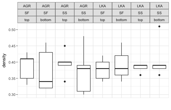
We start with a plot that has three levels of facets.

enter image description here

Now we'll cover the top two facet strips with spanning strips so that we don't have repeated strip labels:

pg = ggplotGrob(p)

# Add spanning strip labels for species
pos = c(4,11)    
for (i in 1:2) {
  pg <- gtable_add_grob(pg, 
                        list(rectGrob(gp=gpar(col="grey50", fill="grey90")),
                             textGrob(unique(densityAGRLKA$species)[i], 
                                      gp=gpar(cex=0.8))), t=3,l=pos[i],b=3,r=pos[i]+7,
                        name=c("a","b"))
}

# Add spanning strip labels for location
pos=c(4,7,11,15)
for (i in 1:4) {
    pg = gtable_add_grob(pg, 
                         list(rectGrob(gp = gpar(col="grey50", fill="grey90")),
                              textGrob(rep(unique(densityAGRLKA$location),2)[i], 
                                       gp=gpar(cex=0.8))), t=4,l=pos[i],b=4,r=pos[i]+3, 
                         name = c("c","d"))
}

grid.draw(pg)

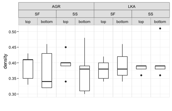
This is what this plot looks like with ggplot2 2.1.0:

enter image description here

However, if I try the same code with ggplot2 2.2.0, I get the original plot back, with no changes to the strip labels. A look at the grob structure of the original plot p suggests why this is happening. I've pasted in the grob tables at the bottom of this question. In order to save space, I've included only the rows related to the facet strips.

Looking at the cells column, note that in the 2.1.0 version of the plot the first two numbers in each row are either 3, 4, or 5, indicating the vertical position of the grob relative to the other grobs in the plot. In the code above, the t and l arguments to gtable_add_grob are set to values of 3 or 4 because those are the facet strip rows that I wanted to cover with spanning strips.

Now look at the cells column in the 2.2.0 version of the plot: Note that the first two numbers are always 6. Also note that the facet strips are comprised of only 8 grobs instead of 24 in version 2.1.0. In version 2.2.0, it seems that each stack of three facet labels is now a single grob instead of three separate grobs. So even if I change the t and b arguments in gtable_add_grob to 6, all three facet strips are covered. Here's an example:

pg = ggplotGrob(p)

# Add spanning strip labels for species
pos = c(4,11)    
for (i in 1:2) {
  pg <- gtable_add_grob(pg, 
                        list(rectGrob(gp=gpar(col="grey50", fill="grey90")),
                             textGrob(unique(densityAGRLKA$species)[i], 
                                      gp=gpar(cex=0.8))), t=6,l=pos[i],b=6,r=pos[i]+7,
                        name=c("a","b"))
}

enter image description here

So, after that very long-winded introduction, here's my question: How can I create spanning facet strips with ggplot2 version 2.2.0 that look like the ones I created using gtable_add_grob with ggplot2 version 2.1.0? I'm hoping there's a simple tweak, but if it requires major surgery, well, that's okay too.

ggplot 2.1.0

pg
TableGrob (9 x 19) "layout": 45 grobs
    z         cells       name                                   grob
2   1 ( 3- 3, 4- 4)  strip-top   absoluteGrob[strip.absoluteGrob.147]
3   2 ( 4- 4, 4- 4)  strip-top   absoluteGrob[strip.absoluteGrob.195]
4   3 ( 5- 5, 4- 4)  strip-top   absoluteGrob[strip.absoluteGrob.243]
5   4 ( 3- 3, 6- 6)  strip-top   absoluteGrob[strip.absoluteGrob.153]
6   5 ( 4- 4, 6- 6)  strip-top   absoluteGrob[strip.absoluteGrob.201]
7   6 ( 5- 5, 6- 6)  strip-top   absoluteGrob[strip.absoluteGrob.249]
8   7 ( 3- 3, 8- 8)  strip-top   absoluteGrob[strip.absoluteGrob.159]
9   8 ( 4- 4, 8- 8)  strip-top   absoluteGrob[strip.absoluteGrob.207]
10  9 ( 5- 5, 8- 8)  strip-top   absoluteGrob[strip.absoluteGrob.255]
11 10 ( 3- 3,10-10)  strip-top   absoluteGrob[strip.absoluteGrob.165]
12 11 ( 4- 4,10-10)  strip-top   absoluteGrob[strip.absoluteGrob.213]
13 12 ( 5- 5,10-10)  strip-top   absoluteGrob[strip.absoluteGrob.261]
14 13 ( 3- 3,12-12)  strip-top   absoluteGrob[strip.absoluteGrob.171]
15 14 ( 4- 4,12-12)  strip-top   absoluteGrob[strip.absoluteGrob.219]
16 15 ( 5- 5,12-12)  strip-top   absoluteGrob[strip.absoluteGrob.267]
17 16 ( 3- 3,14-14)  strip-top   absoluteGrob[strip.absoluteGrob.177]
18 17 ( 4- 4,14-14)  strip-top   absoluteGrob[strip.absoluteGrob.225]
19 18 ( 5- 5,14-14)  strip-top   absoluteGrob[strip.absoluteGrob.273]
20 19 ( 3- 3,16-16)  strip-top   absoluteGrob[strip.absoluteGrob.183]
21 20 ( 4- 4,16-16)  strip-top   absoluteGrob[strip.absoluteGrob.231]
22 21 ( 5- 5,16-16)  strip-top   absoluteGrob[strip.absoluteGrob.279]
23 22 ( 3- 3,18-18)  strip-top   absoluteGrob[strip.absoluteGrob.189]
24 23 ( 4- 4,18-18)  strip-top   absoluteGrob[strip.absoluteGrob.237]
25 24 ( 5- 5,18-18)  strip-top   absoluteGrob[strip.absoluteGrob.285]

ggplot2 2.2.0

pg
TableGrob (11 x 21) "layout": 42 grobs
    z         cells       name                                    grob
28  2 ( 6- 6, 4- 4)  strip-t-1                           gtable[strip]
29  2 ( 6- 6, 6- 6)  strip-t-2                           gtable[strip]
30  2 ( 6- 6, 8- 8)  strip-t-3                           gtable[strip]
31  2 ( 6- 6,10-10)  strip-t-4                           gtable[strip]
32  2 ( 6- 6,12-12)  strip-t-5                           gtable[strip]
33  2 ( 6- 6,14-14)  strip-t-6                           gtable[strip]
34  2 ( 6- 6,16-16)  strip-t-7                           gtable[strip]
35  2 ( 6- 6,18-18)  strip-t-8                           gtable[strip]
Meingoldas answered 22/11, 2016 at 1:49 Comment(2)
I know this question is a bit old these days, but I've used your problem for an example in a related question you might find interesting: https://mcmap.net/q/211978/-nested-facets-in-ggplot2-spanning-groupsPindling
That's great! Thanks for letting me know! I will give facet_nested a try.Meingoldas
P
13

Indeed, ggplot2 v2.2.0 constructs complex strips column by column, with each column a single grob. This can be checked by extracting one strip, then examining its structure. Using your plot:

library(ggplot2)
library(gtable)
library(grid)

# Your data
df = structure(list(location = structure(c(1L, 1L, 1L, 1L, 1L, 1L, 
 1L, 1L, 1L, 1L, 2L, 2L, 2L, 2L, 2L, 2L, 2L, 2L, 2L, 2L, 1L, 1L, 
 1L, 1L, 1L, 1L, 1L, 1L, 1L, 1L, 2L, 2L, 2L, 2L, 2L, 2L, 2L, 2L, 
 2L, 2L), .Label = c("SF", "SS"), class = "factor"), species = structure(c(1L, 
 1L, 1L, 1L, 1L, 1L, 1L, 1L, 1L, 1L, 1L, 1L, 1L, 1L, 1L, 1L, 1L, 
 1L, 1L, 1L, 2L, 2L, 2L, 2L, 2L, 2L, 2L, 2L, 2L, 2L, 2L, 2L, 2L, 
 2L, 2L, 2L, 2L, 2L, 2L, 2L), .Label = c("AGR", "LKA"), class = "factor"), 
    position = structure(c(1L, 1L, 1L, 1L, 1L, 2L, 2L, 2L, 2L, 
    2L, 1L, 1L, 1L, 1L, 1L, 2L, 2L, 2L, 2L, 2L, 1L, 1L, 1L, 1L, 
    1L, 2L, 2L, 2L, 2L, 2L, 1L, 1L, 1L, 1L, 1L, 2L, 2L, 2L, 2L, 
    2L), .Label = c("top", "bottom"), class = "factor"), density = c(0.41, 
    0.41, 0.43, 0.33, 0.35, 0.43, 0.34, 0.46, 0.32, 0.32, 0.4, 
    0.4, 0.45, 0.34, 0.39, 0.39, 0.31, 0.38, 0.48, 0.3, 0.42, 
    0.34, 0.35, 0.4, 0.38, 0.42, 0.36, 0.34, 0.46, 0.38, 0.36, 
    0.39, 0.38, 0.39, 0.39, 0.39, 0.36, 0.39, 0.51, 0.38)), .Names = c("location", 
   "species", "position", "density"), row.names = c(NA, -40L), class = "data.frame")

# Your ggplot with three facet levels
p=ggplot(df, aes("", density)) + 
  geom_boxplot(width=0.7, position=position_dodge(0.7)) + 
  theme_bw() +
  facet_grid(. ~ species + location +  position) +
  theme(panel.spacing=unit(0,"lines"),
     strip.background=element_rect(color="grey30", fill="grey90"),
     panel.border=element_rect(color="grey90"),
     axis.ticks.x=element_blank()) +
  labs(x="")

# Get the ggplot grob
pg = ggplotGrob(p)

# Get the left most strip
index = which(pg$layout$name == "strip-t-1")
strip1 = pg$grobs[[index]]

# Draw the strip
grid.newpage()
grid.draw(strip1)

# Examine its layout
strip1$layout
gtable_show_layout(strip1)

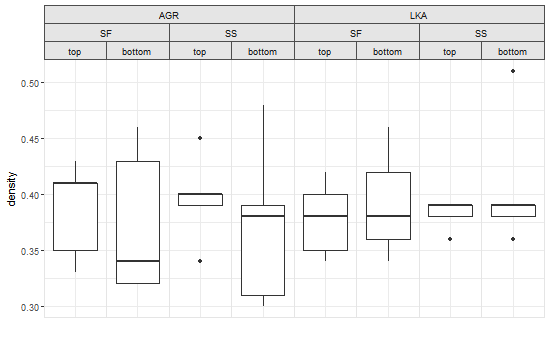
One crude way to get outer strip labels 'spanning' inner labels is to construct the strip from scratch:

# Get the strips, as a list, from the original plot
strip = list()
for(i in 1:8) {
   index = which(pg$layout$name == paste0("strip-t-",i))
   strip[[i]] = pg$grobs[[index]]
}

# Construct gtable to contain the new strip
newStrip  = gtable(widths = unit(rep(1, 8), "null"), heights = strip[[1]]$heights)

## Populate the gtable    
# Top row
for(i in 1:2) {
   newStrip = gtable_add_grob(newStrip, strip[[4*i-3]][1], 
           t = 1, l = 4*i-3, r = 4*i)
}

# Middle row
for(i in 1:4){
   newStrip = gtable_add_grob(newStrip, strip[[2*i-1]][2], 
         t = 2, l = 2*i-1, r = 2*i)
}

# Bottom row
for(i in 1:8) {
   newStrip = gtable_add_grob(newStrip, strip[[i]][3], 
       t = 3, l = i)
}

# Put the strip into the plot 
# (It could be better to remove the original strip. 
# In this case, with a coloured background, it doesn't matter)
pgNew = gtable_add_grob(pg, newStrip, t = 7, l = 5, r = 19)

# Draw the plot
grid.newpage()
grid.draw(pgNew)

OR using vectorised gtable_add_grob (see the comments):

pg = ggplotGrob(p)

# Get a list of strips from the original plot
strip = lapply(grep("strip-t", pg$layout$name), function(x) {pg$grobs[[x]]})

# Construct gtable to contain the new strip
newStrip  = gtable(widths = unit(rep(1, 8), "null"), heights = strip[[1]]$heights)

## Populate the gtable    
# Top row
cols = seq(1, by = 4, length.out = 2)
newStrip = gtable_add_grob(newStrip, lapply(strip[cols], `[`, 1), t = 1, l = cols, r = cols + 3)

# Middle row
cols = seq(1, by = 2, length.out = 4)
newStrip = gtable_add_grob(newStrip, lapply(strip[cols], `[`, 2), t = 2, l = cols, r = cols + 1)

# Bottom row
newStrip = gtable_add_grob(newStrip, lapply(strip, `[`, 3), t = 3, l = 1:8)

# Put the strip into the plot
pgNew = gtable_add_grob(pg, newStrip, t = 7, l = 5, r = 19)

# Draw the plot
grid.newpage()
grid.draw(pgNew)

enter image description here

Psychognosis answered 28/11, 2016 at 7:7 Comment(7)
FWIW gtable_add_grob is vectorised (from the start I argued it should be called gtable_add_grobs, we'd be seeing fewer for loops)Chemosphere
Thanks Sandy. A question to make sure I understand this: It seems like the main lesson (for me at least) is that you need heights = strip[[1]]$heights to get the height of each strip in the stack of (in this case) three facet strips. That's how you get the right vertical size when you overlay the new spanning grobs. Is that correct?Meingoldas
Is there a way to automate this by programmatically figuring out the span length for each row of facet strips? For example, in this case, the top row has two different values, "AGR" and "LKA" and each spans four facets. The middle row has two sets of two values and each value spans two facets, etc. Is there a way to pull that information from the gtable and turn this into a function that automates the process of creating the new spanning grobs?Meingoldas
First question: That's correct. It was easier to use colour, margins, background, heights, etc from the already-constructed strip.Psychognosis
Second question: This is R so the answer has to be "yes". I'm travelling, and I will not get to it for a day or two.Psychognosis
Sounds good. I've already accepted your answer and awarded the bounty, but I won't complain if you get around to automating the process.Meingoldas
Okay, that was more difficult than I originally thought. I may have over-worked things a bit, but it works on your example, and I've tried it on other data where the sequencing of the rows in the strips is not so even. I've put the function into a new answer.Psychognosis
P
7

EDIT To allow for panels of different widths (i.e., scales = "free_x", space = "free_x").

This attempt takes the original ggplot, extracts some information, then constructs a new grob containing the overlapping strips. The function is not pretty but it works ... so far. It requires plyr to be installed.

library(ggplot2)
library(grid)
library(gtable)


df = structure(list(location = structure(c(1L, 1L, 1L, 1L, 1L, 1L, 
    1L, 1L, 1L, 1L, 2L, 2L, 2L, 2L, 2L, 2L, 2L, 2L, 2L, 2L, 1L, 1L, 
    1L, 1L, 1L, 1L, 1L, 1L, 1L, 1L, 2L, 2L, 2L, 2L, 2L, 2L, 2L, 2L, 
    2L, 2L), .Label = c("SF", "SS"), class = "factor"), species = structure(c(1L, 
    1L, 1L, 1L, 1L, 1L, 1L, 1L, 1L, 1L, 1L, 1L, 1L, 1L, 1L, 1L, 1L, 
    1L, 1L, 1L, 2L, 2L, 2L, 2L, 2L, 2L, 2L, 2L, 2L, 2L, 2L, 2L, 2L, 
    2L, 2L, 2L, 2L, 2L, 2L, 2L), .Label = c("AGR", "LKA"), class = "factor"), 
        position = structure(c(1L, 1L, 1L, 1L, 1L, 2L, 2L, 2L, 2L, 
        2L, 1L, 1L, 1L, 1L, 1L, 2L, 2L, 2L, 2L, 2L, 1L, 1L, 1L, 1L, 
        1L, 2L, 2L, 2L, 2L, 2L, 1L, 1L, 1L, 1L, 1L, 2L, 2L, 2L, 2L, 
        2L), .Label = c("top", "bottom"), class = "factor"), density = c(0.41, 
        0.41, 0.43, 0.33, 0.35, 0.43, 0.34, 0.46, 0.32, 0.32, 0.4, 
        0.4, 0.45, 0.34, 0.39, 0.39, 0.31, 0.38, 0.48, 0.3, 0.42, 
        0.34, 0.35, 0.4, 0.38, 0.42, 0.36, 0.34, 0.46, 0.38, 0.36, 
        0.39, 0.38, 0.39, 0.39, 0.39, 0.36, 0.39, 0.51, 0.38)), .Names = c("location", 
    "species", "position", "density"), row.names = c(NA, -40L), class = "data.frame")

# Begin with a regular ggplot with three facet levels
p=ggplot(df, aes("", density)) + 
  geom_boxplot(width=0.7, position=position_dodge(0.7)) + 
  theme_bw() +
  facet_grid(. ~ species + location + position) +
  theme(panel.spacing=unit(0,"lines"),
        strip.background=element_rect(color="grey30", fill="grey90"),
        panel.border=element_rect(color="grey90"),
        axis.ticks.x=element_blank()) +
  labs(x="")

## The function to get overlapping strip labels
OverlappingStripLabels = function(plot) {

# Get the ggplot grob
g = ggplotGrob(plot)

### Collect some information about the strips from the plot
# Get a list of strips
strip = lapply(grep("strip-t", g$layout$name), function(x) {g$grobs[[x]]})

# Number of strips
NumberOfStrips = sum(grepl(pattern = "strip-t", g$layout$name))

# Number of rows
NumberOfRows = length(strip[[1]])

# Panel spacing and it's unit
plot_theme <- function(p) {
   plyr::defaults(p$theme, theme_get())
}
PanelSpacing = plot_theme(plot)$panel.spacing
unit = attr(PanelSpacing, "unit")

# Map the boundaries of the new strips
Nlabel = vector("list", NumberOfRows)
map = vector("list", NumberOfRows)
for(i in 1:NumberOfRows) {

  for(j in 1:NumberOfStrips) {
   Nlabel[[i]][j] = getGrob(grid.force(strip[[j]][i]), gPath("GRID.text"), grep = TRUE)$label
  }

map[[i]][1] = TRUE
for(j in 2:NumberOfStrips) {
   map[[i]][j] = Nlabel[[i]][j] != Nlabel[[i]][j-1]
   }
}


## Construct gtable to contain the new strip
# Set the widths of the strips, based on widths of the panels and PanelSpacing
panel = subset(g$layout, grepl("panel", g$layout$name), l, drop = TRUE)                       
StripWidth = list()
for(i in seq_along(panel)) StripWidth[[i]] = unit.c(g$width[panel[i]], PanelSpacing)

newStrip  = gtable(widths = unit.c(unit(unlist(StripWidth), c("null", unit)))[-2*NumberOfStrips], 
                   heights = strip[[1]]$heights)


## Populate the gtable  
seqLeft = list()
for(i in 1:NumberOfRows) {  
   Left = which(map[[i]] == TRUE)
   seqLeft[[i]] = if((i-1) < 1) 2*Left - 1 else sort(unique(c(seqLeft[[i-1]], 2*Left - 1))) 
   seqRight = c(seqLeft[[i]][-1] -2, (2*NumberOfStrips-1))
   newStrip = gtable_add_grob(newStrip, lapply(strip[(seqLeft[[i]]+1)/2], `[`, i), t = i, l = seqLeft[[i]], r = seqRight)
}

## Put the strip into the plot
# Get the locations of the original strips
pos = subset(g$layout, grepl("strip-t", g$layout$name), t:r)

## Use these to position the new strip
pgNew = gtable_add_grob(g, newStrip, t = unique(pos$t), l = min(pos$l), r = max(pos$r))

return(pgNew)
}

## Draw the plot
grid.newpage()
grid.draw(OverlappingStripLabels(p))

enter image description here

It probably would not be too difficult to break the function, but I tried it on data where the sequencing of the rows is not so even.

p1 = ggplot(mtcars, aes("", hp)) + 
  geom_boxplot(width=0.7, position=position_dodge(0.7)) + 
  theme_bw() +
  facet_grid(. ~ vs + am + carb, labeller = label_both) +
  theme(panel.spacing=unit(0.2,"lines"),
        strip.background=element_rect(color="grey30", fill="grey90"),
        panel.border=element_rect(color="grey90"),
        axis.ticks.x=element_blank()) +
  labs(x="")

  grid.draw(OverlappingStripLabels(p1))

p2 = ggplot(mtcars, aes("", hp)) + 
  geom_boxplot(width=0.7, position=position_dodge(0.7)) + 
  theme_bw() +
  facet_grid(. ~ vs + carb +  am, labeller = label_both) +
  theme(panel.spacing=unit(0.2,"lines"),
        strip.background=element_rect(color="grey30", fill="grey90"),
        panel.border=element_rect(color="grey90"),
        axis.ticks.x=element_blank()) +
  labs(x="")

 grid.draw(OverlappingStripLabels(p2))


df = structure(list(id = 1:19, 
category1 = c("X", "X", "X", "X", "X", "X", "X", "X", "X", "Y", "Y", "Y", "Y", "Y", "Y", "Y", "Y", "Y", "Y"),
category2 = c(21L, 21L, 21L, 22L, 22L, 22L, 22L, 22L, 22L, 23L, 23L, 23L, 24L, 24L, 24L, 25L, 25L, 26L, 26L), 
category3 = c("C1", "C2", "C3", "D1", "D2", "D3", "D5", "D6", "D7", "E1", "E2", "E3", "F1", "F2", "F3", "G1", "G2", "H1", "H2"), 
freq = c(4L, 7L, 4L, 28L, 20L, 0L, 1L, 4L, 1L, 17L, 33L, 31L, 20L, 20L, 21L, 15L, 18L, 12L, 13L)), 
.Names = c("id", "category1", "category2", "category3", "freq"), class = "data.frame", row.names = c(NA, -19L))

p3 = ggplot(df, aes(category3, freq)) + 
  geom_bar(stat = "identity") + 
  facet_grid(. ~ category1 + category2, scale = "free_x", space = "free_x")

 grid.draw(OverlappingStripLabels(p3))
Psychognosis answered 6/12, 2016 at 1:58 Comment(0)

© 2022 - 2024 — McMap. All rights reserved.