How to detect and calculate angle of a prism from this image?
Asked Answered
D

1

0

I am currently trying to detect the edge of a prism shape materials and find the angle of that shape.

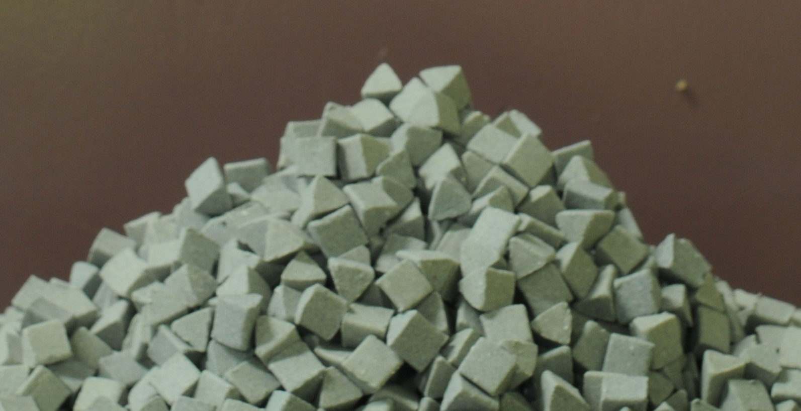
I have an original image like this:

Cone shape material

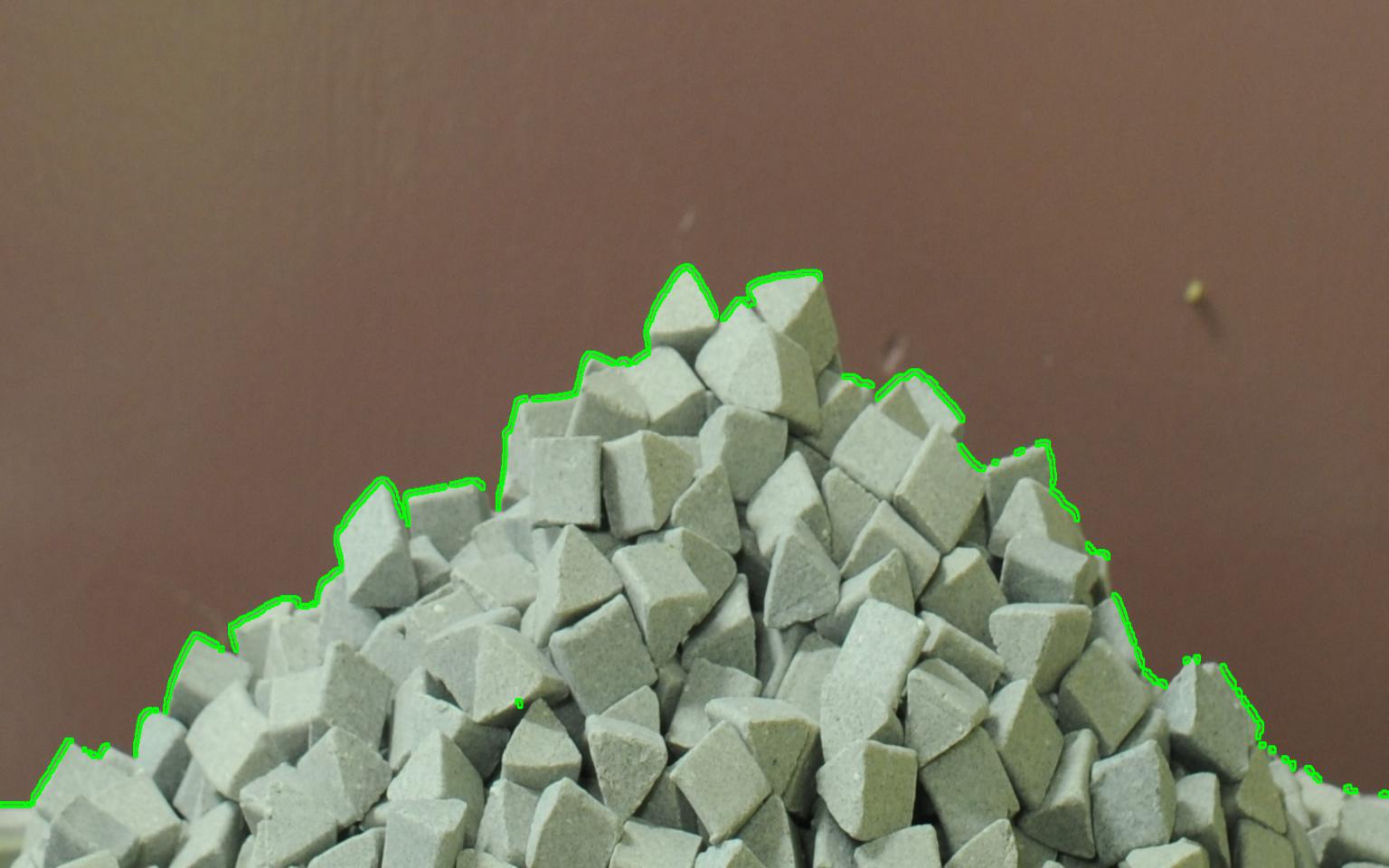
I wrote a Python program that detects the edge between burgundy background and grey materials (the code is given below) and it detects the edges like this:

Processed Image

But I don't know how to find angle from the detected edge. Any ideas?

import glob
import cv2
import numpy as np
import ctypes
import math

def get_screen_resolution():
    user32 = ctypes.windll.user32
    return user32.GetSystemMetrics(0), user32.GetSystemMetrics(1)

def process_photos():
    # Get the list of image files in the directory
    image_files = glob.glob("LEF_*.jpg")

    # Process each image file
    for image_file in image_files:
        process_image(image_file)

def process_image(image_file):
    # Load the image
    image = cv2.imread(image_file)

    # Convert the image to grayscale
    gray = cv2.cvtColor(image, cv2.COLOR_BGR2GRAY)

    # Perform color-based segmentation to extract the burgundy regions
    lower_burgundy = np.array([0, 0, 100])  # Adjust the lower threshold for burgundy color
    upper_burgundy = np.array([100, 100, 255])  # Adjust the upper threshold for burgundy color
    mask = cv2.inRange(image, lower_burgundy, upper_burgundy)

    # Apply a Gaussian blur to the mask to reduce noise
    blurred_mask = cv2.GaussianBlur(mask, (5, 5), 0)

    # Perform Canny edge detection on the grayscale image
    edges_gray = cv2.Canny(gray, 50, 150)

    # Combine the edges with the burgundy regions using bitwise AND
    combined_edges = cv2.bitwise_and(edges_gray, blurred_mask)

    # Dilate the edges to enhance connectivity
    dilated = cv2.dilate(combined_edges, None, iterations=2)

    # Find contours of the edges
    contours, _ = cv2.findContours(dilated.copy(), cv2.RETR_EXTERNAL, cv2.CHAIN_APPROX_SIMPLE)

    # Approximate the contours to straight lines
    lines = cv2.HoughLinesP(dilated, rho=1, theta=np.pi/180, threshold=100, minLineLength=100, maxLineGap=10)

    # Draw the lines on the original image
    if lines is not None:
        # Compute the mean line from the detected line segments
        mean_x1, mean_y1, mean_x2, mean_y2 = np.mean(lines[:, 0, :], axis=0, dtype=np.int32)

        # Draw the mean line
        cv2.line(image, (mean_x1, mean_y1), (mean_x2, mean_y2), (0, 255, 0), 2)

        # Compute the angle of the mean line
        angle = math.atan2(mean_y2 - mean_y1, mean_x2 - mean_x1) * 180 / np.pi
        print("Angle:", angle)

    # Draw the contours on the original image
    cv2.drawContours(image, contours, -1, (0, 255, 0), 2)

    # Resize the image to fit the screen resolution
    screen_width, screen_height = get_screen_resolution()
    image = cv2.resize(image, (screen_width, screen_height))

    # Display the processed image
    cv2.imshow("Processed Image", image)
    cv2.waitKey(0)
    cv2.destroyAllWindows()

process_photos()


Deandra answered 19/5, 2023 at 1:56 Comment(2)
Fitting a polyline consisting of only two lines to edge points directly may be one way. For example, defining the polyline with 3 points (0,y0) - (x1,y1) - (image width,y2), degree of freedom is only 4.Bathesda
sequel to this question is there: #76313731Overseer
R
1

I had a try at this, using some different techniques so you can use and adapt and merge any aspects you like with your own approach.

Notably, I used:

  • cv.inRange() to detect and segment the burgundy background rather than cv.findContours(),
  • a low-pass filter to smooth the "rock" edges and find the peak of the cone,
  • split the image into two sides according to the peak location
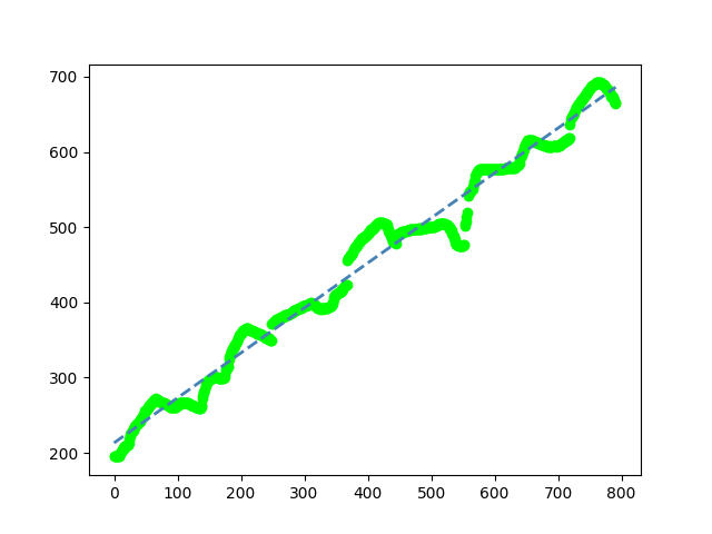
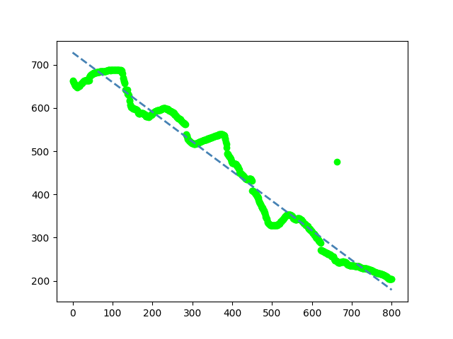
  • fitted a straight line to each side.

 #!/usr/bin/env python3

import cv2 as cv
import numpy as np
from scipy import ndimage
import math

def lowpass(isignal, w):
   # Low pass filter
   # isignal is the input signal
   # osignal is the output signal
   # w is the window width that decides how many pixels affect the output
   kernel = np.lib.pad(np.linspace(1,3,w), (0,w-1), 'reflect') 
   kernel = np.divide(kernel,np.sum(kernel))
   osignal = ndimage.convolve(isignal, kernel) 
   return osignal

# Load image
im = cv.imread('mountain.jpg')
h, w = im.shape[:2]

# Convert to HSV and segment burgundy background
HSV = cv.cvtColor(im, cv.COLOR_BGR2HSV)

# Low and high HSV threshold for background
bglo = np.uint8([5,30,0])
bghi = np.uint8([30,255,255])
bg = cv.inRange(HSV, bglo, bghi)
# Save just for debug, easy cleanup with: rm DEBUG-*png
cv.imwrite('DEBUG-bg.png', bg)

# Get distance from top of image to first black pixel in each col
coltops = (bg!=255).argmax(axis=0)
# Get distance from bottom of last black pixel in each col
y = h - coltops

# Smooth the the curve, I chose image width/10 as the window size - you can experiment
ysmooth = lowpass(y, int(w/10))
for x in range(im.shape[1]):                             # illustration only - can be deleted
   # Plot smooth curve in red on top of original image   # illustration only - can be deleted
   im[h-ysmooth[x],x] = [0,0,255]                        # illustration only - can be deleted
cv.imwrite('DEBUG-smooth.png', im)                       # illustration only - can be deleted

# Now locate the x-coordinate of the peak of the smoothed curve to get the mountain centre
cx = ysmooth.argmax() # prints 792
print(f'DEBUG: x-coordinate of mountain centre is {cx}')

# Now split original (not smoothed) y-values into two separate lines - left and right side
yLeft = y[:cx]
yRight = y[cx:]

import matplotlib.pyplot as plt                                    # illustration only - can be deleted

# Fit straight line to left side
x = np.arange(len(yLeft))
a, b = np.polyfit(x, yLeft, 1)
angle = math.degrees(math.atan(a))
print(f'Left side: y = {a:0.3f} * x + {b:0.3f}, => angle: {angle:0.3f}')

# Plot the points
plt.scatter(x, yLeft, color='lime')                                # illustration only - can be deleted

# Draw line of best fit to plot
plt.plot(x, a*x+b, color='steelblue', linestyle='--', linewidth=2) # illustration only - can be deleted
plt.savefig('left.png')                                            # illustration only - can be deleted
plt.clf() # clear for right side                                   # illustration only - can be deleted

# Fit straight line to right side
x = np.arange(len(yRight))
a, b = np.polyfit(x, yRight, 1)
angle = math.degrees(math.atan(a))
print(f'Right side: y = {a:0.3f} * x + {b:0.3f}, => angle: {angle:0.3f}')

# Plot the points
plt.scatter(x, yRight, color='lime')                              # illustration only - can be deleted

# Draw line of best fit to plot
plt.plot(x, a*x+b, color='steelblue', linestyle='--', linewidth=2)# illustration only - can be deleted
plt.savefig('right.png')                                          # illustration only - can be deleted

You can safely ignore all the matplotlib.pyplot stuff - it is just for illustration.

It outputs this:

Left side: y = 0.598 * x + 213.244, => angle: 30.873
Right side: y = -0.687 * x + 728.566, => angle: -34.492

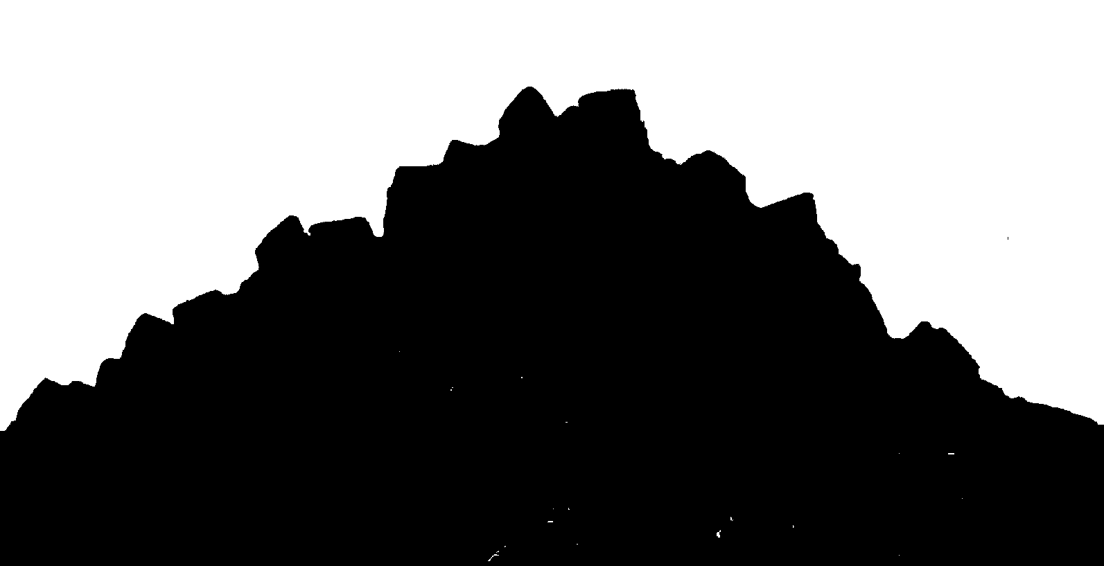
The segmented background (DEBUG-bg.png) looks like this:

enter image description here

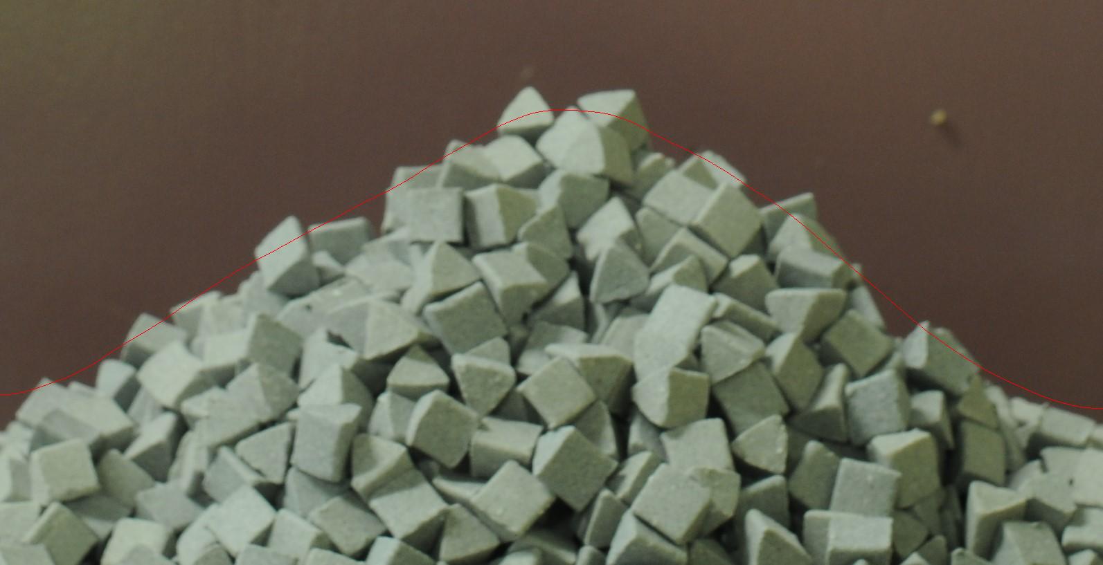
The smoothed edges (DEBUG-smooth.png) look like this:

enter image description here

And the left and right sides plotted look like this:

enter image description here

enter image description here

Romine answered 19/5, 2023 at 10:16 Comment(0)

© 2022 - 2024 — McMap. All rights reserved.