Applying Cost Functions in R

Question

I am in the beginning stages of machine learning in R and I find it hard to believe that there are no packages to solving the cost function for different types of regression algorithms. For example, if I want to solve the cost function for a logistic regression, the manual way would be below:

https://www.r-bloggers.com/logistic-regression-with-r-step-by-step-implementation-part-2/

# Implement Sigmoid function
sigmoid <- function(z)
{
g <- 1/(1+exp(-z))
return(g)
}

#Cost Function
cost <- function(theta)
{
m <- nrow(X)
g <- sigmoid(X%*%theta)
J <- (1/m)*sum((-Y*log(g)) - ((1-Y)*log(1-g)))
return(J)
}

##Intial theta
initial_theta <- rep(0,ncol(X))

#Cost at inital theta
cost(initial_theta)

In the glm function is there a way to automatically do this? Or for each algorithm that I apply, do I need to manually do it like this?

Guilford

No don't have to for example see help page of glmnet function from package glmnet i.e. library(glmnet);x=matrix(rnorm(100*20),100,20);g2=sample(1:2,100,replace=TRUE);fit2=glmnet(x,g2,family="binomial") – Rhizomorphous

Answer 1

We could use optim for optimization or use glm directly

set.seed(1)
X <- matrix(rnorm(1000), ncol=10) # some random data
Y <- sample(0:1, 100, replace=TRUE)

# Implement Sigmoid function
sigmoid <- function(z) {
  g <- 1/(1+exp(-z))
  return(g)
}

cost.glm <- function(theta,X) {
  m <- nrow(X)
  g <- sigmoid(X%*%theta)
  (1/m)*sum((-Y*log(g)) - ((1-Y)*log(1-g)))
}

X1 <- cbind(1, X)
optim(par=rep(0,ncol(X1)), fn = cost.glm, method='CG',
      X=X1, control=list(trace=TRUE))
#$par 
#[1] -0.067896075 -0.102393236 -0.295101743  0.616223350  0.124031764  0.126735986 -0.029509039 -0.008790282  0.211808300 -0.038330703 -0.210447146
#$value
#[1] 0.6255513
#$counts
#function gradient 
#      53       28 

glm(Y~X, family=binomial)$coefficients
# (Intercept)           X1           X2           X3           X4           X5           X6           X7           X8           X9          X10 
#-0.067890451 -0.102411613 -0.295104858  0.616228141  0.124017980  0.126737807 -0.029523206 -0.008790988  0.211810613 -0.038319484 -0.210445717 

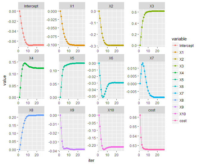
The figure below shows how the cost and the coefficients iteratively computed with optim converge to the ones computed with glm.

Capacious

How did you get all the coefficients' values that you use for the plot? – Selinaselinda

@Selinaselinda control=list(trace=TRUE) in optim shows the intermediate values of all the coefficients. – Capacious

@SandipanDey How do you go from the printed values to the numbers shown in the plot for all the variables? Can you show me with some code how you went from optim to the values? Thanks. – Selinaselinda