How can I obtain segmented linear regressions with a priori breakpoints?

Question

I need to explain this in excruciating detail because I don't have the basics of statistics to explain in a more succinct way. Asking here in SO because I am looking for a python solution, but might go to stats.SE if more appropriate.

I have downhole well data, it might be a bit like this:

Rt      T
0.0000  15.0000
4.0054  15.4523
25.1858 16.0761
27.9998 16.2013
35.7259 16.5914
39.0769 16.8777
45.1805 17.3545
45.6717 17.3877
48.3419 17.5307
51.5661 17.7079
64.1578 18.4177
66.8280 18.5750
111.1613    19.8261
114.2518    19.9731
121.8681    20.4074
146.0591    21.2622
148.8134    21.4117
164.6219    22.1776
176.5220    23.4835
177.9578    23.6738
180.8773    23.9973
187.1846    24.4976
210.5131    25.7585
211.4830    26.0231
230.2598    28.5495
262.3549    30.8602
266.2318    31.3067
303.3181    37.3183
329.4067    39.2858
335.0262    39.4731
337.8323    39.6756
343.1142    39.9271
352.2322    40.6634
367.8386    42.3641
380.0900    43.9158
388.5412    44.1891
390.4162    44.3563
395.6409    44.5837

(the Rt variable can be considered a proxy for depth, and T is temperature). I also have 'a priori' data giving me the temperature at Rt=0 and, not shown, some markers that i can use as breakpoints, guides to breakpoints, or at least compare to any discovered breakpoints.

The linear relationship of these two variables is in some depth intervals affected by some processes. A simple linear regression is

q, T0, r_value, p_value, std_err = stats.linregress(Rt, T)

and looks like this, where you can see the deviations clearly, and the poor fit for T0 (which should be 15):

I want to be able to perform a series of linear regressions (joining at ends of each segment), but I want to do it: (a) by NOT specifying the number or locations of breaks, (b) by specifying the number and location of breaks, and (c) calculate the coefficients for each segment

I think I can do (b) and (c) by just splitting the data up and doing each bit separately with a bit of care, but I don't know about (a), and wonder if there's a way someone knows this can be done more simply.

I have seen this: https://stats.stackexchange.com/a/20210/9311, and I think MARS might be a good way to deal with it, but that's just because it looks good; I don't really understand it. I tried it with my data in a blind cut'n'paste way and have the output below, but again, I don't understand it:

Lewendal

Answer 1

The short answer is that I solved my problem using R to create a linear regression model, and then used the segmented package to generate the piecewise linear regression from the linear model. I was able to specify the expected number of breakpoints (or knots) n as shown below using psi=NA and K=n.

The long answer is:

R version 3.0.1 (2013-05-16)
Platform: x86_64-pc-linux-gnu (64-bit)

# example data:
bullard <- structure(list(Rt = c(5.1861, 10.5266, 11.6688, 19.2345, 59.2882, 
68.6889, 320.6442, 340.4545, 479.3034, 482.6092, 484.048, 485.7009, 
486.4204, 488.1337, 489.5725, 491.2254, 492.3676, 493.2297, 494.3719, 
495.2339, 496.3762, 499.6819, 500.253, 501.1151, 504.5417, 505.4038, 
507.6278, 508.4899, 509.6321, 522.1321, 524.4165, 527.0027, 529.2871, 
531.8733, 533.0155, 544.6534, 547.9592, 551.4075, 553.0604, 556.9397, 
558.5926, 561.1788, 562.321, 563.1831, 563.7542, 565.0473, 566.1895, 
572.801, 573.9432, 575.6674, 576.2385, 577.1006, 586.2382, 587.5313, 
589.2446, 590.1067, 593.4125, 594.5547, 595.8478, 596.99, 598.7141, 
599.8563, 600.2873, 603.1429, 604.0049, 604.576, 605.8691, 607.0113, 
610.0286, 614.0263, 617.3321, 624.7564, 626.4805, 628.1334, 630.9889, 
631.851, 636.4198, 638.0727, 638.5038, 639.646, 644.8184, 647.1028, 
647.9649, 649.1071, 649.5381, 650.6803, 651.5424, 652.6846, 654.3375, 
656.0508, 658.2059, 659.9193, 661.2124, 662.3546, 664.0787, 664.6498, 
665.9429, 682.4782, 731.3561, 734.6619, 778.1154, 787.2919, 803.9261, 
814.335, 848.1552, 898.2568, 912.6188, 924.6932, 940.9083), Tem = c(12.7813, 
12.9341, 12.9163, 14.6367, 15.6235, 15.9454, 27.7281, 28.4951, 
34.7237, 34.8028, 34.8841, 34.9175, 34.9618, 35.087, 35.1581, 
35.204, 35.2824, 35.3751, 35.4615, 35.5567, 35.6494, 35.7464, 
35.8007, 35.8951, 36.2097, 36.3225, 36.4435, 36.5458, 36.6758, 
38.5766, 38.8014, 39.1435, 39.3543, 39.6769, 39.786, 41.0773, 
41.155, 41.4648, 41.5047, 41.8333, 41.8819, 42.111, 42.1904, 
42.2751, 42.3316, 42.4573, 42.5571, 42.7591, 42.8758, 43.0994, 
43.1605, 43.2751, 44.3113, 44.502, 44.704, 44.8372, 44.9648, 
45.104, 45.3173, 45.4562, 45.7358, 45.8809, 45.9543, 46.3093, 
46.4571, 46.5263, 46.7352, 46.8716, 47.3605, 47.8788, 48.0124, 
48.9564, 49.2635, 49.3216, 49.6884, 49.8318, 50.3981, 50.4609, 
50.5309, 50.6636, 51.4257, 51.6715, 51.7854, 51.9082, 51.9701, 
52.0924, 52.2088, 52.3334, 52.3839, 52.5518, 52.844, 53.0192, 
53.1816, 53.2734, 53.5312, 53.5609, 53.6907, 55.2449, 57.8091, 
57.8523, 59.6843, 60.0675, 60.8166, 61.3004, 63.2003, 66.456, 
67.4, 68.2014, 69.3065)), .Names = c("Rt", "Tem"), class = "data.frame", row.names = c(NA, 
-109L))


library(segmented)  # Version: segmented_0.2-9.4

# create a linear model
out.lm <- lm(Tem ~ Rt, data = bullard)

# Set X breakpoints: Set psi=NA and K=n:
o <- segmented(out.lm, seg.Z=~Rt, psi=NA, control=seg.control(display=FALSE, K=3))
slope(o)  # defaults to confidence level of 0.95 (conf.level=0.95)

# Trickery for placing text labels
r <- o$rangeZ[, 1]
est.psi <- o$psi[, 2]
v <- sort(c(r, est.psi))
xCoord <- rowMeans(cbind(v[-length(v)], v[-1]))
Z <- o$model[, o$nameUV$Z]
id <- sapply(xCoord, function(x) which.min(abs(x - Z)))
yCoord <- broken.line(o)[id]

# create the segmented plot, add linear regression for comparison, and text labels
plot(o, lwd=2, col=2:6, main="Segmented regression", res=TRUE)
abline(out.lm, col="red", lwd=1, lty=2)  # dashed line for linear regression
text(xCoord, yCoord, 
    labels=formatC(slope(o)[[1]][, 1] * 1000, digits=1, format="f"), 
    pos = 4, cex = 1.3)

Lewendal

Answer 2

What you want is technically called spline interpolation, particularly order-1 spline interpolation (which would join straight line segments; order-2 joins parabolas, etc).

There is already a question here on Stack Overflow dealing with Spline Interpolation in Python, which will help you on your question. Here's the link. Post back if you have further questions after trying those tips.

Shantay

I don't understand how I can use the methods in the linked question. I am quite dim when it comes to this, so perhaps you could explain a bit more? I have irregularly-spaced 1D data and I want to perform some linear regression analysis on it; the linked question is about point interpolation of regularly-gridded multivariate data: 2D, 3D?? – Lewendal

@a different ben: Oops, my bad. A quick Google search revealed that Scipy has spline interpolation. I never used it, but see if the material in this link helps you: docs.scipy.org/doc/scipy/reference/tutorial/interpolate.html – Shantay

Answer 3

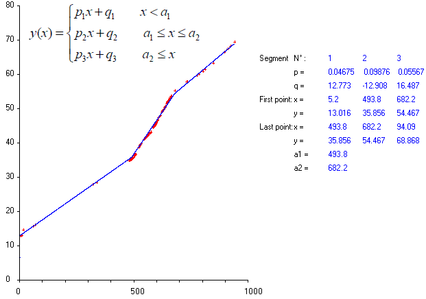
A very simple method ( not iterative, without initial guess, no bound to specify) is provided pages 30-31 in the paper : https://fr.scribd.com/document/380941024/Regression-par-morceaux-Piecewise-Regression-pdf . The result is :

NOTE : The method is based on the fitting of an integral equation. The present exemple is not a favourable case because the distribution of the abscisses of the points is far to be regular (no points in large ranges). This makes the numerical integration less accurate. Nevertheless, the piecewise fitting is surprisingly not bad.

Fishery