simultaneously update theta0 and theta1 to calculate gradient descent in python

I am taking the machine learning course from coursera. There is a topic called gradient descent to optimize the cost function. It says to simultaneously update theta0 and theta1 such that it will minimize the cost function and will reach to global minimum.

The formula for gradient descent is

How do i do this programmatically using python? I am using numpy array and pandas to start from scratch to understand step by step its logic.

For now i have only calculated cost function

# step 1 - collect our data
data = pd.read_csv("datasets.txt", header=None)

def compute_cost_function(x, y, theta):
    '''
        Taking in a numpy array x, y, theta and generate the cost function
    '''
    m = len(y)
    # formula for prediction = theta0 + theta1.x
    predictions = x.dot(theta)
    # formula for square error = ((theta1.x + theta0) - y)**2
    square_error = (predictions - y)**2
    # sum of square error function
    return 1/(2*m) * np.sum(square_error)

# converts into numpy represetation of the pandas dataframe. The axes labels will be excluded
numpy_data = data.values
m = data[0].size
x = np.append(np.ones((m, 1)), numpy_data[:, 0].reshape(m, 1), axis=1)
y = numpy_data[:, 1].reshape(m, 1)
theta = np.zeros((2, 1))

compute_cost_function(x, y, theta)

def gradient_descent(x, y, theta, alpha):
    '''
        simultaneously update theta0 and theta1 where 
        theta0 = theta0 - apha * 1/m * (sum of square error)
    '''
    pass

I know i have to call that compute_cost_function from gradient descent but could not apply that formula.

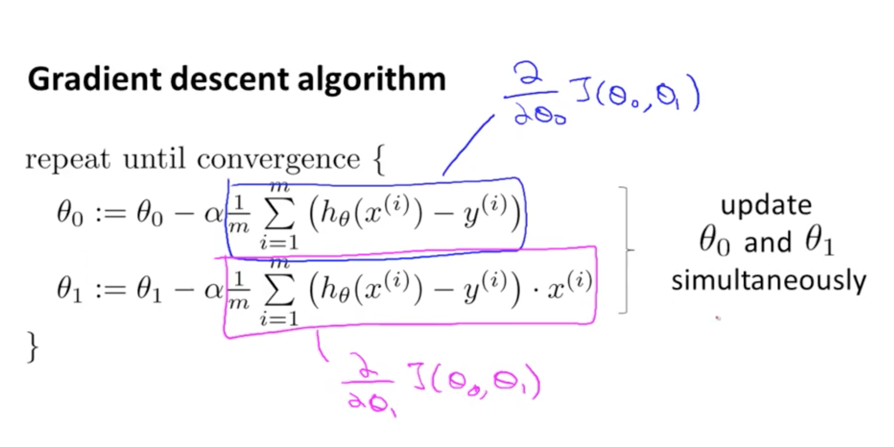
What it means is that you use the previous values of the parameters and compute what you need on the right hand side. Once you're done, update the parameters. To do this the most clearly, create a temporary array inside your function that stores the results on the right hand side and return the computed result when you're finished.

def gradient_descent(x, y, theta, alpha):
    ''' simultaneously update theta0 and theta1 where
        theta0 = theta0 - apha * 1/m * (sum of square error) ''' 
    theta_return = np.zeros((2, 1))
    theta_return[0] = theta[0] - (alpha / m) * ((x.dot(theta) - y).sum())
    theta_return[1] = theta[1] - (alpha / m) * (((x.dot(theta) - y)*x[:, 1][:, None]).sum())

    return theta_return

We first declare the temporary array then compute each part of the parameters, namely the intercept and slope separately then return what we need. The nice thing about the above code is that we're doing it vectorized. For the intercept term, x.dot(theta) performs matrix vector multiplication where you have your data matrix x and parameter vector theta. By subtracting this result with the output values y, we are computing the sum over all errors between the predicted values and true values, then multiplying by the learning rate then dividing by the number of samples. We do something similar with the slope term only we additionally multiply by each input value without the bias term. We additionally need to ensure the input values are in columns as slicing along the second column of x results in a 1D NumPy array instead of a 2D with a singleton column. This allows the elementwise multiplication to play nicely together.

One more thing to note is that you don't need to compute the cost at all when updating the parameters. Mind you, inside your optimization loop it'll be nice to call it as you're updating your parameters so you can see how well your parameters are learning from your data.

To make this truly vectorized and thus exploiting the simultaneous update, you can formulate this as a matrix-vector multiplication on the training examples alone:

def gradient_descent(x, y, theta, alpha):
    ''' simultaneously update theta0 and theta1 where
        theta0 = theta0 - apha * 1/m * (sum of square error) ''' 
    return theta - (alpha / m) * x.T.dot(x.dot(theta) - y)

What this does is that when we compute x.dot(theta), this calculates the the predicted values, then we combine this by subtracting with the expected values. This produces the error vector. When we pre-multiply by the transpose of x, what ends up happening is that we take the error vector and perform the summation vectorized such that the first row of the transposed matrix x corresponds to values of 1 meaning that we are simply summing up all of the error terms which gives us the update for the bias or intercept term. Similarly the second row of the transposed matrix x additionally weights each error term by the corresponding sample value in x (without the bias term of 1) and computes the sum that way. The result is a 2 x 1 vector which gives us the final update when we subtract with the previous value of our parameters and weighted by the learning rate and number of samples.

I didn't realize you were putting the code in an iterative framework. In that case you need to update the parameters at each iteration.

def gradient_descent(x, y, theta, alpha, iterations):

    ''' simultaneously update theta0 and theta1 where
    theta0 = theta0 - apha * 1/m * (sum of square error) ''' 

    theta_return = np.zeros((2, 1))
    for i in range(iterations):
        theta_return[0] = theta[0] - (alpha / m) * ((x.dot(theta) - y).sum())
        theta_return[1] = theta[1] - (alpha / m) * (((x.dot(theta) - y)*x[:, 1][:, None]).sum())
        theta = theta_return

    return theta

theta = gradient_descent(x, y, theta, 0.01, 1000)

At each iteration, you update the parameters then set it properly so that the next time, the current updates become the previous updates.

Recommended topics

Hot tags