How to calculate one-sided tolerance interval with scipy

Question

I would like to calculate a one sided tolerance bound based on the normal distribution given a data set with known N (sample size), standard deviation, and mean.

If the interval were two sided I would do the following:

conf_int = stats.norm.interval(alpha, loc=mean, scale=sigma)

In my situation, I am bootstrapping samples, but if I weren't I would refer to this post on stackoverflow: Correct way to obtain confidence interval with scipy and use the following: conf_int = stats.norm.interval(0.68, loc=mean, scale=sigma / np.sqrt(len(a)))

How would you do the same thing, but to calculate this as a one sided bound (95% of values are above or below x<--bound)?

Repentant

None of the other scipy stats functions are useful? The docs should have a ling to the source for those functions - maybe you can repurpose one of them with minor changes. – Jasper

See accepted answer - as far as I know none of the other functions would fit this problem but I would love to know about it if that changes or if I overlooked a function that would work for this problem. – Repentant

Answer 1

I assume that you are interested in computing one-side tolerance bound using the normal distribution (based on the fact you mention the scipy.stats.norm.interval function as the two-sided equivalent of your need).

Then the good news is that, based on the tolerance interval Wikipedia page:

One-sided normal tolerance intervals have an exact solution in terms of the sample mean and sample variance based on the noncentral t-distribution.

(FYI: Unfortunately, this is not the case for the two-sided setting)

This assertion is based on this paper. Besides paragraph 4.8 (page 23) provides the formulas.

The bad news is that I do not think there is a ready-to-use scipy function that you can safely tweak and use for your purpose.

But you can easily calculate it yourself. You can find on Github repositories that contain such a calculator from which you can find inspiration, for example that one from which I built the following illustrative example:

import numpy as np
from scipy.stats import norm, nct

# sample size
n=1000

# Percentile for the TI to estimate
p=0.9
# confidence level
g = 0.95

# a demo sample
x = np.array([np.random.normal(100) for k in range(n)])

# mean estimate based on the sample
mu_est = x.mean()

# standard deviation estimated based on the sample
sigma_est = x.std(ddof=1)

# (100*p)th percentile of the standard normal distribution
zp = norm.ppf(p)

# gth quantile of a non-central t distribution
# with n-1 degrees of freedom and non-centrality parameter np.sqrt(n)*zp
t = nct.ppf(g, df=n-1., nc=np.sqrt(n)*zp)

# k factor from Young et al paper
k = t / np.sqrt(n)

# One-sided tolerance upper bound
conf_upper_bound = mu_est + (k*sigma_est)

Dialectologist

Thank you so much! You are correct, I was looking for a one-sided tolerance bound using the normal distribution - post edited. I somehow didn't realize that two sided vs lower/upper bound differed so greatly mathematically and this is a very helpful example!! Thank you for the detail on this response – Repentant

@Greta, you can consider accepting the answer if it addressed you question. stackoverflow.com/help/someone-answers. comments might get deleted, and it would help if someone faces a similar problem – Fatso

Answer 2

Here is a one-line solution with the openturns library, assuming your data is a numpy array named sample.

import openturns as ot
ot.NormalFactory().build(sample.reshape(-1, 1)).computeQuantile(0.95)

Let us unpack this. NormalFactory is a class designed to fit the parameters of a Normal distribution (mu and sigma) on a given sample: NormalFactory() creates an instance of this class.

The method build does the actual fitting and returns an object of the class Normal which represents the normal distribution with parameters mu and sigma estimated from the sample.

The sample reshape is there to make sure that OpenTURNS understands that the input sample is a collection of one-dimension points, not a single multi-dimensional point.

The class Normal then provides the method computeQuantile to compute any quantile of the distribution (the 95-th percentile in this example).

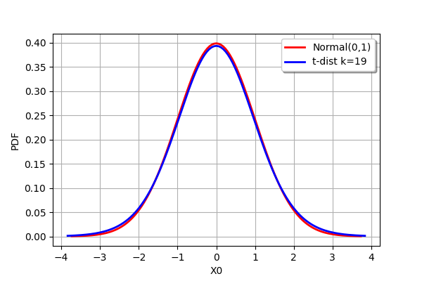
This solution does not compute the exact tolerance bound because it uses a quantile from a Normal distribution instead of a Student t-distribution. Effectively, that means that it ignores the estimation error on mu and sigma. In practice, this is only an issue for really small sample sizes.

To illustrate this, here is a comparison between the PDF of the standard normal N(0,1) distribution and the PDF of the Student t-distribution with 19 degrees of freedom (this means a sample size of 20). They can barely be distinguished.

deg_freedom = 19
graph = ot.Normal().drawPDF()
student = ot.Student(deg_freedom).drawPDF().getDrawable(0)
student.setColor('blue')
graph.add(student)
graph.setLegends(['Normal(0,1)', 't-dist k={}'.format(deg_freedom)])
graph

Yare

Hello and thank you for commenting. Can you clarify and let me know if this is a onesided output? – Repentant

Yes, 95% of all values are below the given bound. – Yare