Preliminaries
Some preliminary code:
%matplotlib inline
import numpy as np
import cv2
from matplotlib import pyplot as plt
from skimage.morphology import extrema
from skimage.morphology import watershed as skwater

def ShowImage(title,img,ctype):
  plt.figure(figsize=(10, 10))
  if ctype=='bgr':
    b,g,r = cv2.split(img)       # get b,g,r
    rgb_img = cv2.merge([r,g,b])     # switch it to rgb
    plt.imshow(rgb_img)
  elif ctype=='hsv':
    rgb = cv2.cvtColor(img,cv2.COLOR_HSV2RGB)
    plt.imshow(rgb)
  elif ctype=='gray':
    plt.imshow(img,cmap='gray')
  elif ctype=='rgb':
    plt.imshow(img)
  else:
    raise Exception("Unknown colour type")
  plt.axis('off')
  plt.title(title)
  plt.show()
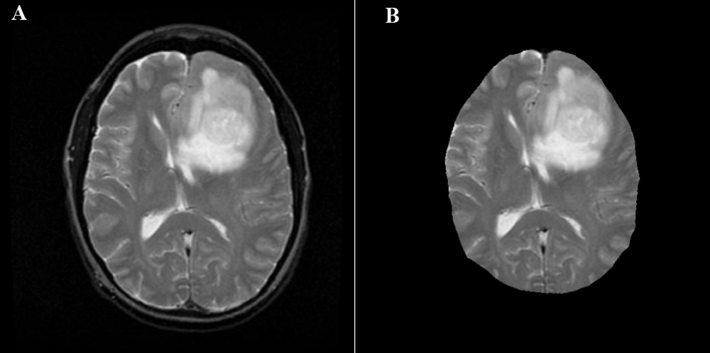
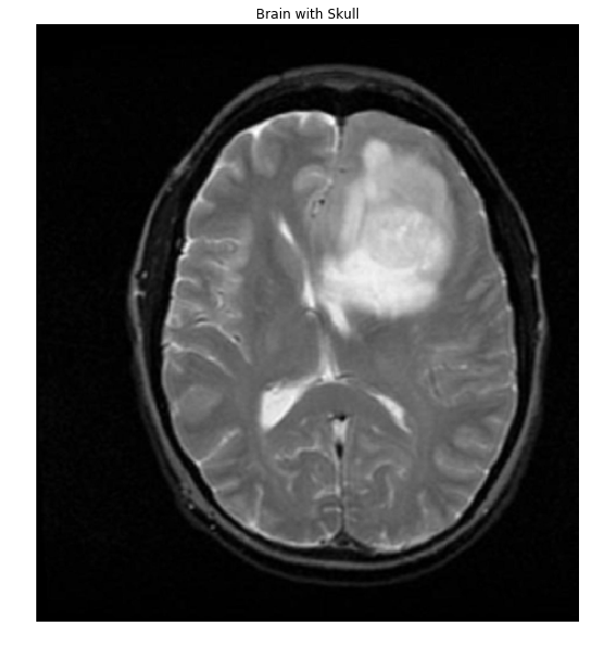
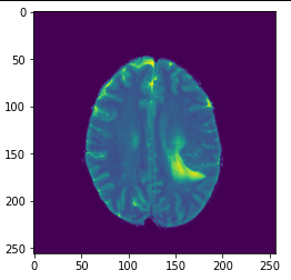
For reference, here's one of the brain+skulls you linked to:
#Read in image
img           = cv2.imread('brain.png')
gray          = cv2.cvtColor(img,cv2.COLOR_BGR2GRAY)
ShowImage('Brain with Skull',gray,'gray')
![Brain with Skull]()
Extracting a Mask
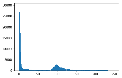
If the pixels in the image can be classified into two different intensity classes, that is, if they have a bimodal histogram, then Otsu's method can be used to threshold them into a binary mask. Let's check that assumption.
#Make a histogram of the intensities in the grayscale image
plt.hist(gray.ravel(),256)
plt.show()
![Histogram]()
Okay, the data is nicely bimodal. Let's apply the threshold and see how we do.
#Threshold the image to binary using Otsu's method
ret, thresh = cv2.threshold(gray,0,255,cv2.THRESH_OTSU)
ShowImage('Applying Otsu',thresh,'gray')
![Tresholded brain+skull]()
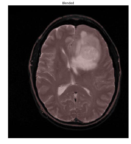
Things are easier to see if we overlay our mask onto the original image
colormask = np.zeros(img.shape, dtype=np.uint8)
colormask[thresh!=0] = np.array((0,0,255))
blended = cv2.addWeighted(img,0.7,colormask,0.1,0)
ShowImage('Blended', blended, 'bgr')
![Mask overlaid on brain+skull]()
Extracting the Brain
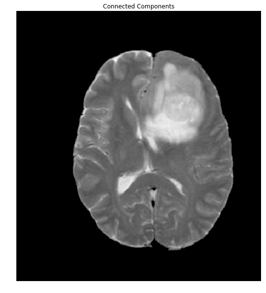
The overlap of the brain (shown in red) with the mask is so perfect, that we'll stop right here. To do so, let's extract the connected components and find the largest one, which will be the brain.
ret, markers = cv2.connectedComponents(thresh)

#Get the area taken by each component. Ignore label 0 since this is the background.
marker_area = [np.sum(markers==m) for m in range(np.max(markers)) if m!=0]
#Get label of largest component by area
largest_component = np.argmax(marker_area)+1 #Add 1 since we dropped zero above
#Get pixels which correspond to the brain
brain_mask = markers==largest_component

brain_out = img.copy()
#In a copy of the original image, clear those pixels that don't correspond to the brain
brain_out[brain_mask==False] = (0,0,0)
ShowImage('Connected Components',brain_out,'rgb')
![Brain extracted with connected components]()
Considering the Second Brain
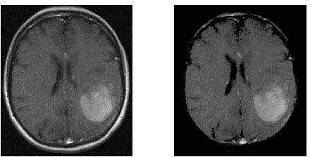
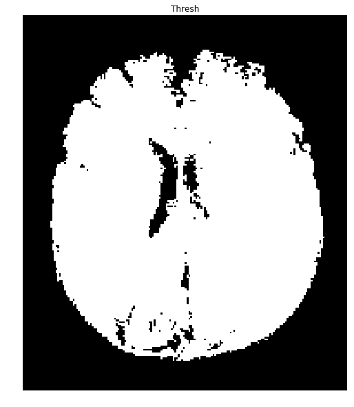
Running this again with your second image produces a mask with many holes:
![Second Brain]()
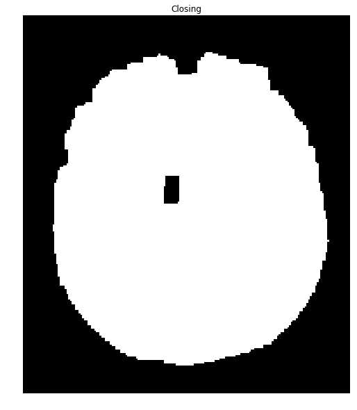
We can close many of these holes using a closing transformation:
brain_mask = np.uint8(brain_mask)
kernel = np.ones((8,8),np.uint8)
closing = cv2.morphologyEx(brain_mask, cv2.MORPH_CLOSE, kernel)
ShowImage('Closing', closing, 'gray')
![Brain mask with holes closed]()
We can now extract the brain:
brain_out = img.copy()
#In a copy of the original image, clear those pixels that don't correspond to the brain
brain_out[closing==False] = (0,0,0)
ShowImage('Connected Components',brain_out,'rgb')
![Second brain with better mask]()
If you need to cite this for some reason:
Richard Barnes. (2018). Using Otsu's method for skull-brain segmentation (v1.0.1). Zenodo. https://doi.org/10.5281/zenodo.6042312

